A credit score may need to explain why an applicant’s income or age affects a lending decision. Discretization groups values into bins so risk teams can compare default rates, build interpretable scorecards, and reduce sensitivity to noise and extreme values. Bin boundaries are modeling decisions: they must preserve useful risk signals while remaining stable and defensible to auditors. section 4.4.2 section 4.4
Choose granularity before assigning scores:
- Fine classing uses many narrow intervals. It can capture subtle patterns when each bin has enough observations, but sparse bins raise overfitting and maintenance risks. section 4.4.2
- Coarse classing combines observations into fewer broad groups. It is simpler to explain and often more stable, but may hide differences in risk. section 4.4.2
- Review missing values, sentinel codes, and outliers separately. A dedicated missing or outlier bin may retain information that imputation or ordinary intervals would conceal. section 4.4.4
Quantile-bin a numeric credit feature
A manual Python workflow fills missing numeric values with the feature median, then calls `pd.qcut(values, 10, duplicates='drop', retbins=True)`. It saves the resulting edges and counts events and nonevents in each bin before calculating Weight of Evidence (WoE) and Information Value (IV). Ten bins are a starting setting, not a reason to skip inspection: duplicate edges can reduce the bin count, and manual coarse classing may still be appropriate. section 5.3.3
Listing 6.1 Creating the BinningProcess and specifying selection criteria
from optbinning import BinningProcess, Scorecard
from optbinning.scorecard import plot_auc_roc, plot_cap, plot_ks
from sklearn.linear_model import LogisticRegression

print("Starting OptBinning demonstration with the same BFSI dataset...")

selection_criteria = {
    "iv": {                    #1
        "min": 0.025,
        "max": 0.7,
        "strategy": "highest",
        "top": 20
    },
    "quality_score": {    #2
        "min": 0.01
    }
}

binning_process = BinningProcess(     #3
    variable_names=feature_list,
    categorical_variables=cat_features,
    selection_criteria=selection_criteria
)

binning_process.fit(X, y)    #4
print("BinningProcess fit completed.")
For automated numeric and categorical binning, `BinningProcess` fits on a feature matrix and target. The listing shows IV bounds, a top-20 selection rule, and a minimum quality score; these constraints make feature selection explicit rather than binning every column indiscriminately. section 6.1.1
Figure 6.1 Default rate and bin counts for D_68_last. Each bar represents the number of observations per bin, broken down by event and nonevent. The black line shows the default rate for each bin. Bars labeled Bin Special represent outliers or special codes (e.g., -999), while Bin Missing indicates null values handled separately.
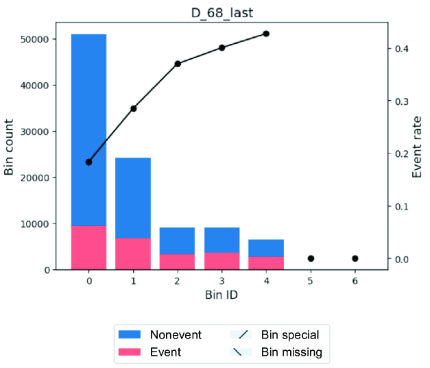
Inspect bin counts alongside default rates before accepting a split. The figure distinguishes ordinary intervals from special-code and missing-value bins, making sparse groups and unexpected risk trends easier to spot. section 6.1.1
Keep the chosen boundaries consistent when scoring new applicants, and review them as distributions change. WoE and IV connect bins to scorecard feature assessment; Population Stability Index (PSI) monitoring helps flag shifts that warrant investigation. Document treatments for missing or extreme values, particularly when they may affect fairness or regulatory review. section 6.6 section 4.4.4




