Binning converts continuous or detailed values into discrete intervals or categories. It prepares numeric data for outlier detectors that rely on histograms or categorical features. section 3.2.4 section 9.6
Choose a binning method to fit the outlier-detection task:
- Use equal-width bins generally for univariate outliers, where the count in each bin can indicate how rare a value is. section 9.6
- Use equal-count bins generally for multivariate outliers, focusing on rare combinations while assuming univariate outliers are tested elsewhere. section 9.6
- Check sensitivity to extreme values and bin count: equal-width bins can compress ordinary values into edge bins, leave gaps, or hide an outlier among inliers. section 9.6
Interpretable categories for expense records
An outlier-detection example converts dates to day-of-month categories, times to hour categories, and amounts to categories based on their number of digits. These choices make the resulting frequent-itemset analysis more interpretable. section 3.2.4
Figure 9.1 The effect of the number of bins. In the first row we see where 20 bins are used and in the second row, 50 bins. In each row we see a distribution of uniform data with no outliers (left pane), with a single outlier with value 3.0 (middle pane), and with a second outlier with value 100.0 (right pane). In the top-right pane we see, using 20 bins, the 3.0 value is placed in a bin with inliers. In the bottom-right pane we see, using 50 bins, the 3.0 value is in a separate bin with low count so will be recognized as an outlier.
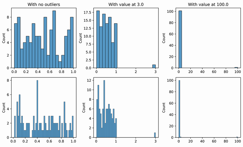
Compare how 20 versus 50 equal-width bins place uniform data and outliers at 3.0 and 100.0; the example shows how bin count can change whether an outlier shares a bin with inliers. section 9.6




