A cumulative distribution function (CDF) gives the probability that a random variable X is no greater than a threshold x: F(x) = P(X ≤ x). It turns a distribution into answers to questions such as “What is the chance of at most two absences?” For a < b, subtract cumulative probabilities to find P(a < X ≤ b) = F(b) − F(a). section 2.3.3 section 9.3.2
How the CDF is built and read:
- For a discrete variable, add the probabilities of every outcome up to and including x: F(x) = Σₖ≤ₓ P(X = k). Its graph steps upward at possible outcomes and stays flat between them. section 2.4.3
- For a continuous variable, accumulate probability under its density up to x. A normal distribution produces an S-shaped CDF; a PDF value alone is not a probability for a range. section 2.3.3 section 3.1.1
- A CDF never decreases and remains between 0 and 1. At a discrete outcome, its value includes that outcome’s probability. section 2.3.3 section 2.4.3
Add probabilities for a discrete threshold
For the sum of two six-sided dice, the probabilities of totals 2, 3, and 4 are 0.0278, 0.0556, and 0.0833. Thus F(4) = 0.0278 + 0.0556 + 0.0833 ≈ 0.167: the chance of a total no greater than 4 is about 16.7%. section 2.4.3
Calculate a normal interval in Python
For a standard normal variable, SciPy gives F(1) ≈ 0.84134 and F(1.5) ≈ 0.93319. Subtract to get about 0.09185, or 9.18%, between 1 and 1.5. from scipy.stats import norm probability = norm.cdf(1.5) - norm.cdf(1) print(probability * 100) # about 9.18 section 3.1.1
For call-center absentee counts modeled with a Poisson distribution at λ = 2, cumulative probabilities for zero, at most one, and at most two absences are 13.53%, 40.60%, and 67.67%. Compute a table with `poisson.cdf(k_values, lam)` or add the individual probabilities in order; the final cumulative probability should reach 1 when all possible outcomes are included. section 9.3.2
Figure 9.2 A Poisson distribution and its cumulative distribution, with the bars representing the Poisson probabilities and the line representing the cumulative probabilities. The bars correspond to the primary y axis on the left, whereas the line with circular markers corresponds to the secondary y axis on the right.
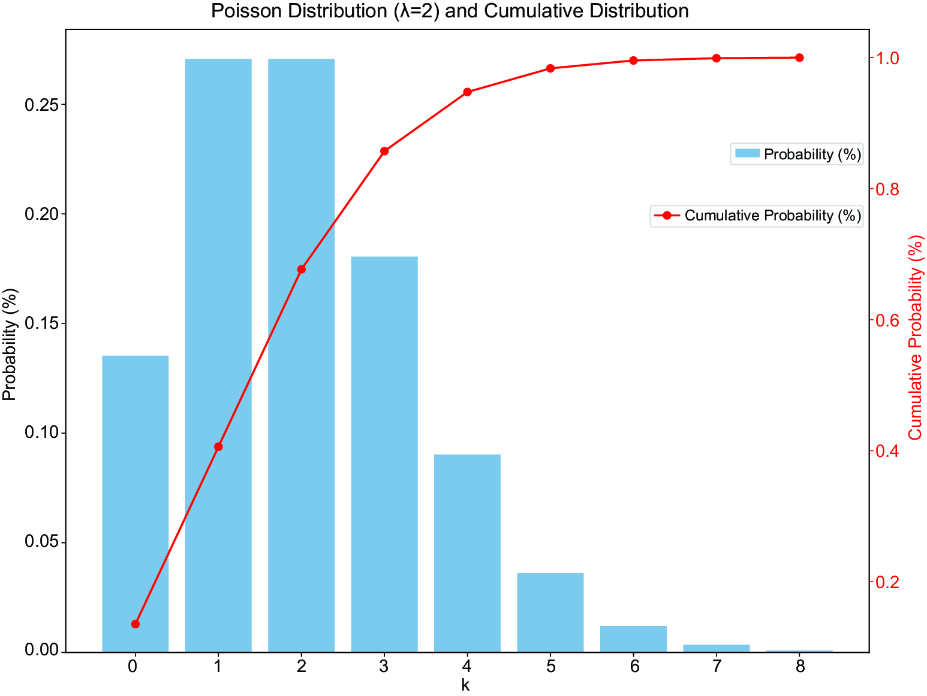
Compare each bar’s individual Poisson probability with the line’s accumulated probability at the same absentee count. section 9.3.2
In Monte Carlo simulation, cumulative probabilities define intervals that map random numbers to outcomes. Choose and parameterize the underlying distribution using data, domain knowledge, or explicit assumptions. If a simulation uses only a truncated set of outcomes, normalize its probabilities to sum to 1 before sampling. section 9.2 section 9.4



