A cumulative distribution function (CDF) turns a value on a probability distribution into the area to its left: the probability from negative infinity up to that value. This is useful because a probability density value—the height of a curve at one point—is not itself a probability for a continuous measurement. section 3.8 section 4.5
To find the probability that a value falls between two bounds, calculate the CDF at the upper bound and subtract the CDF at the lower bound: F(upper) − F(lower). The remaining area is the probability for that interval. section 3.8 section 4.5
Success rate between 0.4 and 0.7
For a beta distribution with 7 successes and 3 failures, `beta.cdf(.7, 7, 3)` gives 0.4628 and `beta.cdf(.4, 7, 3)` gives 0.0250. Their difference, about 0.4378, means a 43.78% chance that the underlying success rate is in the 0.4–0.7 range. section 3.8
Golden retriever weights
With a normal distribution whose mean is 64 pounds and standard deviation is 3 pounds, `norm.cdf(63, 64, 3) - norm.cdf(61, 64, 3)` is 0.2108. That area represents a 21.08% probability that a golden retriever weighs between 61 and 63 pounds. section 4.5
A CDF helps keep three related ideas separate:
- A probability density is the curve height at a value; it is mainly useful for plotting or, with calculus, finding areas. section 3.8 section 4.5
- A cumulative probability is the area from the left tail up to one chosen value. section 4.5
- An interval probability is the area between two values, found by subtracting cumulative areas. section 3.8
Figure 4.9 Subtracting areas using the CDF to get a middle range of area/probability
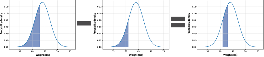
The shaded middle region shows why subtracting two left-side cumulative areas leaves exactly the probability between the lower and upper bounds. section 4.5
CDFs apply across probability distributions, including beta and normal distributions. In SciPy, distribution-specific methods such as `beta.cdf()` and `norm.cdf()` perform the area calculation without manually using integrals. section 3.8 section 4.12



