Free energy calculation estimates how a molecular change affects thermodynamic free energy, especially the binding affinity of a ligand for a target protein. It is particularly useful during lead optimization, when promising hits are refined into candidates with stronger binding and fewer off-target effects. section 9.3 section 9.3.1
The method uses statistical mechanics, force fields, molecular-dynamics sampling, and high-performance computing to estimate binding-related free-energy changes. Predictive accuracy near 1 kcal/mol can guide potency optimization while reducing the compounds that require synthesis and experimental testing. section 9.3.1
A Free Energy Perturbation (FEP) workflow typically proceeds as follows:
- Morph one ligand into another and run molecular-dynamics simulations to estimate the free energy of transformation. section 9.3.1
- Use a lower estimated free energy as a signal of higher binding affinity. section 9.3.1
- For active learning, featurize molecules, sample an initial diverse set, run free energy calculations, train a surrogate model, and select further molecules within a computation budget. section 9.3.1
Figure 9.8 Multi-stage active learning pipeline for structure-based lead optimization using free energy perturbation (FEP) calculations. The workflow begins with a large molecule library (10M-1B compounds) that is filtered down to 10K-1M molecules using machine learning ADMET models. From this filtered set, an initial sample of 500-1K diverse compounds undergoes medium-fidelity FEP evaluation (~1 day of computation). These results train a surrogate model that rapidly scores 10K-1M molecules to identify promising candidates. Based on these predictions, 500 molecules are strategically sampled for high-fidelity FEP analysis (1-2 days), resulting in approximately 10 synthesized hit molecules that advance to subsequent development stages. The diagram illustrates how computational resources (purple) are efficiently allocated to increasingly smaller but higher-quality compound sets (orange), enabling exploration of vast chemical spaces while concentrating expensive physics-based calculations on the most promising candidates.
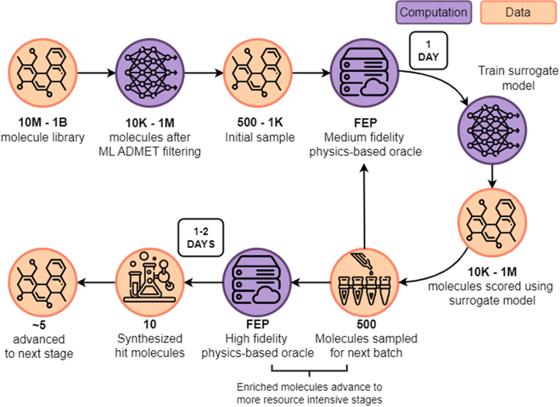
Shows how active learning allocates increasingly expensive FEP calculations across large molecular libraries, from initial medium-fidelity evaluation through high-fidelity selection and synthesis. section 9.3.1
