A Gaussian process (GP) is a probability distribution over functions. For any finite choice of inputs x₁,…,xₙ, the function values (f(x₁),…,f(xₙ)) have a joint Gaussian distribution. A mean function μ(x) specifies their expected values; a positive-definite kernel κ(x,x′) specifies their covariance. Observed input–target pairs update this prior over functions to a posterior used for regression predictions. section 6.5 section 6.7
For training inputs X and test inputs X*, form K = κ(X,X), K* = κ(X,X*), and K** = κ(X*,X*). Under the noiseless-observation assumption, the joint Gaussian distribution of training and test outputs can be conditioned on observed targets y. Its posterior mean is μ(X*) + K*ᵀK⁻¹(y − μ(X)); its posterior covariance is K** − K*ᵀK⁻¹K*. The mean supplies predictions, while the covariance describes uncertainty across the chosen test points. These expressions use Gaussian conditioning rather than fitting one fixed function. section 6.5 section 6.6
A from-scratch regression implementation follows the covariance calculation:
- Choose a mean function and kernel. One implementation uses a zero mean and a radial basis function kernel, exp(−‖x−z‖²/(2L²)), with length scale L. section 6.5
- Evaluate the kernel on training–training, training–test, and test–test input pairs to construct K, K*, and K**. section 6.5
- Condition the joint Gaussian on the observed targets to compute the posterior mean and covariance at test inputs. section 6.5
Continuous-value prediction
Predicting atmospheric CO₂ levels from measurements illustrates the regression task; the worked implementation assumes a sinusoidal model and uses a radial basis function kernel. Samples from the prior and posterior make the effect of conditioning on observations visible. section 6.0 section 6.5
A GP can also model an unknown performance function in Bayesian optimization. As evaluations accumulate, its posterior informs which continuous hyperparameters to try next: expected improvement or a GP upper confidence bound balances promising results against uncertainty. Applications include searches over support vector machine and random forest classifier settings. section 7.4.1
Listing 6.4 Gaussian process regression
import numpy as np
import matplotlib.pyplot as plt
from scipy.spatial.distance import cdist

np.random.seed(42)

class GPreg:

 def __init__(self, X_train, y_train, X_test):

     self.L = 1.0
     self.keps = 1e-8

     self.muFn = self.mean_func(X_test)
     self.Kfn = self.kernel_func(X_test, X_test) + 1e-15*np.eye(
      np.size(X_test))

     self.X_train = X_train
     self.y_train = y_train
     self.X_test = X_test

 def mean_func(self, x):
     muFn = np.zeros(len(x)).reshape(-1,1)
     return muFn

 def kernel_func(self, x, z):
     sq_dist = cdist(x/self.L, z/self.L, 'euclidean')**2
     Kfn = 1.0 * np.exp(-sq_dist/2)
     return Kfn

 def compute_posterior(self):
     K = self.kernel_func(self.X_train, self.X_train)
     Ks = self.kernel_func(self.X_train, self.X_test)
     Kss = self.kernel_func(self.X_test, self.X_test) + self
      .keps*np.eye(np.size(self.X_test))
     Ki = np.linalg.inv(K) #1

     postMu = self.mean_func(self.X_test) + np.dot(np.transpose(Ks),
      np.dot(Ki, (self.y_train - self.mean_func(self.X_train))))
     postCov = Kss - np.dot(np.transpose(Ks), np.dot(Ki, Ks))

     self.muFn = postMu
     self.Kfn = postCov

     return None

 def generate_plots(self, X, num_samples=3):
     plt.figure()
     for i in range(num_samples):
         fs = self.gauss_sample(1)
         plt.plot(X, fs, '-k')
         #plt.plot(self.X_train, self.y_train, 'xk')

     mu = self.muFn.ravel()
     S2 = np.diag(self.Kfn)
     plt.fill(np.concatenate([X, X[::-1]]), np.concatenate([mu –
      2*np.sqrt(S2), (mu + 2*np.sqrt(S2))[::-1]]), alpha=0.2, fc='b')
     plt.show()

 def gauss_sample(self, n):      #2
     A = np.linalg.cholesky(self.Kfn)
     Z = np.random.normal(loc=0, scale=1, size=(len(self.muFn),n))
     S = np.dot(A,Z) + self.muFn       #3
     return S

def main():

    # generate noise-less training data
    X_train = np.array([-4, -3, -2, -1, 1])
    X_train = X_train.reshape(-1,1)
    y_train = np.sin(X_train)

    # generate  test data
    X_test = np.linspace(-5, 5, 50)
    X_test = X_test.reshape(-1,1)

    gp = GPreg(X_train, y_train, X_test)
    gp.generate_plots(X_test,3)   #4
    gp.compute_posterior()
    gp.generate_plots(X_test,3)   #5


if __name__ == "__main__":
    main()
Inspect the regression implementation’s mean and kernel functions alongside its posterior computation. section 6.5
Figure 6.8 Gaussian process regression: Samples from the prior (left) and posterior (right)
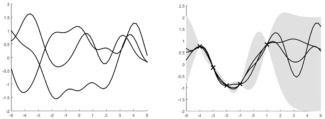
Compare sampled functions before and after observations update the prior. section 6.5


