Graph convolutional network

As explained in Optimization Algorithms: AI techniques for design, planning, and control problems

A graph convolutional network is a neural network that aggregates information from graph neighborhoods to compute node, edge, or graph representations and predictions.

A graph convolutional network (GCN) learns representations from node features and the edges connecting nodes. Rather than describing each node in isolation, it uses information from local neighborhoods. This makes GCNs an inductive graph-embedding method: a learned function can produce representations for nodes that were not present during training. section 11.3.1

Figure 11.6 Message passing and updating in GCN

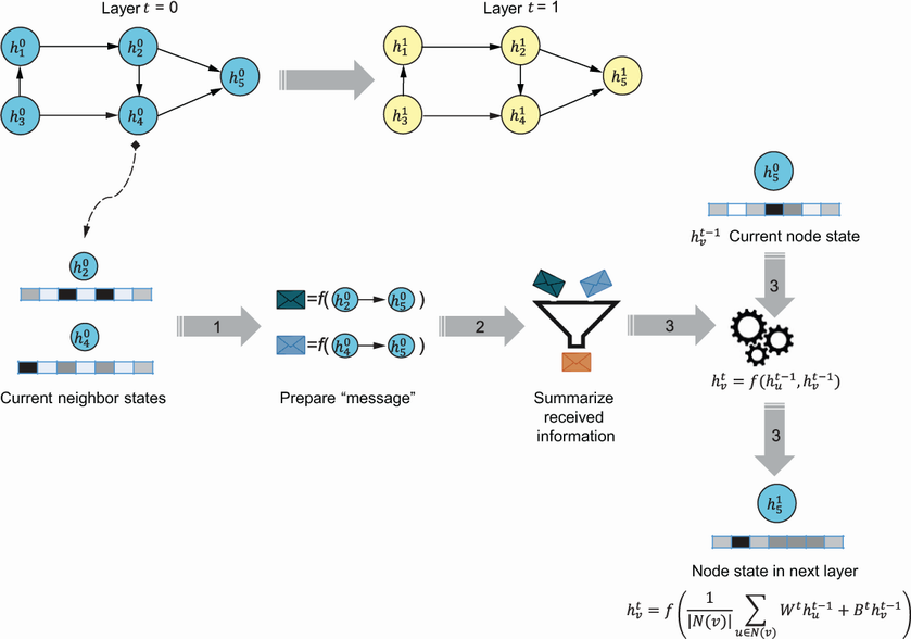
The message-passing diagram shows the central intuition: connected nodes contribute information as node representations are updated. section 11.3.1

Node representations with PyTorch Geometric

A Cora example loads node features and edges, then passes them through two GCNConv layers. ReLU and dropout separate the layers; the second layer produces outputs sized to the dataset’s classes. Training uses the labeled nodes selected by a training mask. The example connects neighborhood aggregation to a practical node-learning task without requiring a hand-built convolution layer. section 11.3.1

For the traveling salesman problem, a GCN can serve as the representation-learning stage of a larger pipeline. Node features and an adjacency matrix define the graph; message passing creates a low-dimensional embedding; a multilayer perceptron predicts which nodes or edges belong to a solution. Graph search then uses those probabilities to seek a feasible tour. The predictions do not, by themselves, guarantee one. section 11.7

Supervised training can compare predictions with optimal tours supplied by a solver such as Concorde. Training a TSP model from scratch requires substantial preprocessing and code, so the practical TSP demonstration loads a pretrained model. Treat that demonstration as an example of the wider graph-learning pipeline, not as evidence that its particular pretrained model is a GCN. section 11.7

How Optimization Algorithms: AI techniques for design, planning, and control problems covers it

How deep it goes

Explains inductive neighborhood embedding and illustrates a two-layer implementation, but defers from-scratch TSP training in favor of a pretrained-model demonstration.

Examples

Uses a Cora node-learning implementation and a traveling-salesman pipeline with a separate pretrained graph-learning demonstration.

What it assumes

Introduces machine-learning fundamentals and graph embedding before the GCN example, while practical code assumes familiarity with Python model training.

What you can do after

Apply it via PyTorch Geometric to construct a two-layer node-learning model; evaluate/understand its role in a TSP prediction-and-search pipeline.

How it connects

Connects graph embedding and message passing to multilayer perceptrons, supervised learning, and graph search.

liveBookmanning.com

Read Optimization Algorithms: AI techniques for design, planning, and control problems on liveBook Get the book at manning.com

Also explained in

• 

  liveBookmanning.com
  Graph Neural Networks in ActionA convolutional graph neural network is a class of graph neural network architectures that use convolution-like neighborhood aggregation.
• 

  liveBookmanning.com
  Knowledge Graphs and LLMs in ActionA graph convolutional network is a graph-neural-network model that updates node representations by aggregating information from graph neighborhoods.
• 

  liveBookmanning.com
  Machine Learning Algorithms in DepthA graph convolutional network is a graph neural network that computes node representations by aggregating information from graph neighborhoods.

Compare how 4 books explain graph convolutional network →

Related concepts

• GraphSAGEcontrasts with · GraphSAGE is an inductive graph-neural-network method that learns node representations by sampling and aggregating information from node neighborhoods.
• graph neural networkkind of · A graph neural network is a neural-network model that learns representations or predictions from graph-structured data by combining information from connected entities.
• graphuses · A graph is a mathematical structure consisting of vertices connected by edges that represent relationships or connections.
• graph attention networkcontrasts with · A graph attention network is a graph neural network that uses attention weights to aggregate information from neighboring nodes, allowing their contributions to differ.

This explainer was generated by Manning's knowledge graph from the text of Optimization Algorithms: AI techniques for design, planning, and control problems. The section links point to the parts of the book it draws on.