A hidden state is a fixed-size tensor that summarizes the sequence processed so far. At time t, an RNN combines the previous state hₜ₋₁ with the current input xₜ to produce hₜ. Reusing the same computation at every step lets one model process sequences of different lengths. section 4.1.2 section 4.6
The recurrent update
The implementation pattern is: initialize history_summary to zero, loop over each input, compute new_summary = RNN(history_summary, inputs[t]), and replace the old state. For a sequence of T items, the final state hT represents the last item together with preceding items. With T = 3, the unrolled states are h₀, h₁, h₂, and h₃; h₀ is an all-zero vector. section 4.1.2
The state carries information forward and can also pass upward to later layers. In sequence-to-sequence models, the encoder’s final state hT initializes the decoder instead of a zero vector. This transfers a summary of the input sequence into decoding and allows gradients to connect the decoder with the encoder. section 4.6 section 11.3
A simple RNN stores information in one repeatedly transformed state: the current input and previous state are concatenated, passed through a linear layer and tanh, and emitted as the next hidden activation. Long sequences make this fixed representation difficult to optimize because gradients traverse many repeated operations. LSTMs address this limitation by pairing hₜ with a context state Cₜ and regulating information through forget, input, and output gates. section 6.6.1 section 6.6.2
Figure 4.4 Diagram of the RNN process. We use t to represent the current point in time (the tth item in a sequence). The RNN takes in a single representation of all previous content ht − 1 and information about the newest item in the sequence xt. The RNN merges these into a new representation of everything seen so far ht, and the process repeats until we reach the end of the sequence.
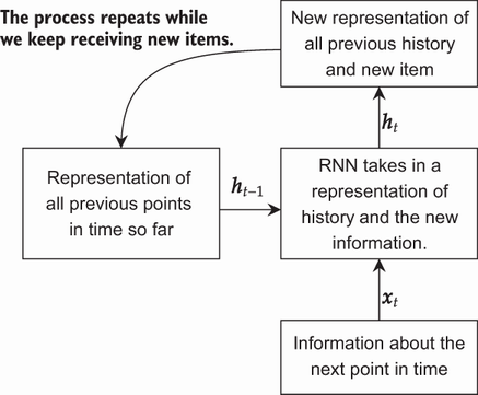
Use the recurrent-process diagram to trace how hₜ₋₁ and xₜ merge into hₜ across the sequence. section 4.1.2