A hyperplane turns one linear equation into geometry. In two dimensions it is a line; in three dimensions it is a plane; in higher dimensions it is the flat shape described by one equation with any number of variables. This viewpoint makes a linear system easier to picture: each equation contributes one hyperplane. section 3.1.1
Write a hyperplane as a1x1 + a2x2 + … + aNxN + aN+1 = 0, or equivalently a1x1 + a2x2 + … + aNxN = b. The variable coefficients determine its orientation, while the free coefficient shifts it. Multiplying every coefficient by the same nonzero number leaves the represented hyperplane unchanged. section 3.1.1 section 3.5.3
Solving a system means finding where its hyperplanes meet. N hyperplanes in N-dimensional space can meet at one point, giving one solution. Parallel hyperplanes have no common point; coincident hyperplanes share every point on the same geometric object, producing infinitely many solutions. These cases correspond to equations that are dependent except for, or including, the free coefficient. section 3.1.2 section 3.1.3
Two trains, one intersection
Two linear equations in two unknowns can be drawn as two route lines. Their crossing is the coordinate pair that solves both equations—for example, the point (300, 150). The same idea scales: three planes can identify a point in 3D without needing to visualize every higher-dimensional case. section 3.1.1 section 3.1.2
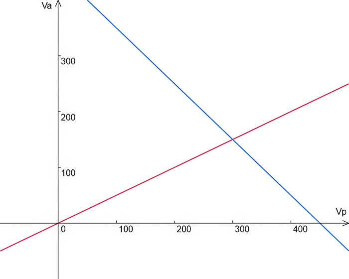
Use the route-line diagram to connect simultaneous equations with the practical task of locating one shared position. section 3.1.1
The geometry also explains useful system behaviors:
- Overspecified systems have more equations than variables. They usually lack one exact common intersection, but numerical methods may find a point close enough to all hyperplanes for noisy measurements such as computed tomography. section 3.2.1
- Underspecified systems often have a continuum of solutions. Two nonparallel planes in 3D meet in a line, and that line—not a single coordinate tuple—can be the symbolic answer. section 3.2.2
- Naively constructing an intersection from lower-dimensional intersections grows factorially with dimension, so direct geometric methods become impractical quickly. section 3.4.1
The hyperplane picture is a guide, not a promise that every system has one clean point. For midsize systems, elimination-based methods are recommended; sparse representations can improve performance, while large iterative methods require convergence checks and may need preconditioning. Small symbolic problems can be solved with SymPy. section 3.11





