A decision boundary separates feature-space regions assigned to different classes. For a linear binary classifier, predict the sign of θ·x + θ₀, where x is a feature vector, θ is a weight vector, and θ₀ is an offset. The boundary is the set of points satisfying θ·x + θ₀ = 0: a hyperplane with normal vector θ. Points on the θ side receive label +1; points on the opposite side receive −1. section 5.2
Figure 5.2 Linear classifier a decision boundary
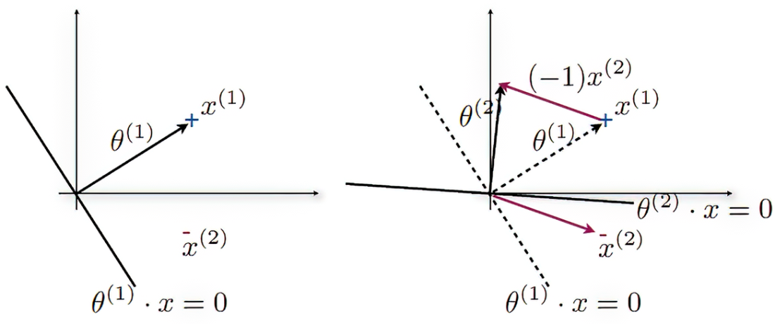
The two-dimensional diagram shows how a line divides the predicted classes and how θ determines its orientation. section 5.2
Correctly separating the training points does not necessarily determine a single boundary: different values of θ and θ₀ can make the same predictions. A support vector machine adds a geometric criterion. For a point x, its distance to the boundary is |θ·x + θ₀| / ||θ||. Choose a correctly classifying boundary that maximizes the smallest such distance across the training points—the margin. This can be posed as a quadratic optimization problem with linear classification constraints and a small-||θ|| objective. section 5.3
Figure 5.8 Max margin solution of SVM classifier
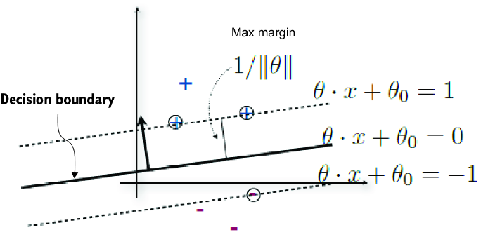
The maximum-margin diagram distinguishes the decision boundary from the margin boundaries pushed outward toward the training points. section 5.3
From labels to a boundary
On the iris dataset, fit a perceptron to binary labels and use the sign of θ·x + θ₀ to predict a class. Compare predictions with ground truth to count mistakes or form a confusion matrix. A maximum-margin classifier instead uses the training points’ distances from the boundary to choose among separating classifiers. section 5.2 section 5.3



