A linear relationship is a pattern between two variables that approximately follows a straight line. As one variable changes, the other tends to change in a consistent direction: both rise together in a positive relationship, or one rises while the other falls in a negative one. The closer the points cluster around a line, the stronger the pattern. section 7.1 section 7.2
Hotter days, more sports drinks
A shop can compare temperature with sports-drink sales across 10 days. Plot temperature on the x-axis and sales on the y-axis: the dots trend upward and roughly follow an unseen line. That suggests a positive linear relationship, making temperature a plausible input for forecasting sales. section 7.1
Figure 7.1 A scatterplot showing 10 data points relating weather temperature to sports drink sales. The points seem to follow a “line” and have an upward trend pattern: as temperature increases, so do sales.
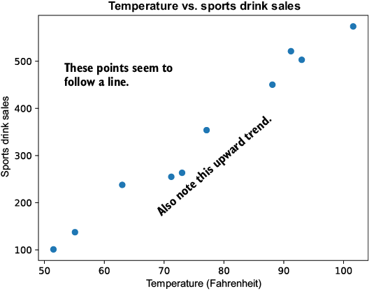
Use the scatterplot to judge the pattern before calculating anything: an upward, roughly straight arrangement suggests a positive linear relationship. section 7.1
A scatterplot is a useful first check, but it does not prove that one variable causes the other. A relationship may be coincidental, affected by other variables, or nonlinear—such as polynomial or exponential—so a straight line would be the wrong description. Common sense and later model testing matter. section 7.1 section 1.7
Pearson correlation summarizes the strength and direction of a linear relationship with r, from -1 to 1. Values near 1 indicate a strong positive pattern; values near -1 indicate a strong negative pattern; values near 0 indicate little linear correlation. For the temperature-and-sales data, r is about 0.9889. section 7.2
When the pattern is suitably linear, linear regression fits a line between input and output variables. That fitted line can predict values not previously seen, but useful predictions depend on the relationship holding up beyond the observed data. section 7.0 section 1.7