Local neighborhood

As explained in Data Without Labels

A neighborhood is the region around a point containing points at a specified distance from that point, represented as an n-sphere in n-dimensional space.

A local neighborhood answers a practical clustering question: which observations are close enough to a chosen point to count as nearby? Represent observations in a vector space, choose a point P and a radius ε greater than zero, and include every point whose distance from P is at most ε. In two dimensions this region is a circle; in three dimensions it is a sphere. section 2.5.1

Figure 2.26 Representation of data points in a vector-space diagram. On the right-side we have a point P, and the circle drawn is of radius ε. So, for ε > 0, the neighborhood of P is defined by the set of points that are at less than or equal to ε distance from the point P.

The circle makes the distance rule visible: points on or inside the radius belong to P’s neighborhood. section 2.5.1

Neighborhoods let density-based clustering compare nearby regions. The number of observations inside a neighborhood acts as its mass; its size determines its volume. Increasing ε increases the volume, but how many additional points it captures depends on the data distribution. Nearby regions with similar, high densities can form a cluster, while sparse regions can separate clusters or contain outliers. Relative density matters more here than a density value on its own. section 2.5.1 section 2.5

DBSCAN turns this idea into a threshold test. It uses ε for the neighborhood radius and minPts for the minimum number of points needed for a dense region. A point is a core point when its ε-neighborhood contains at least minPts observations, counting the point itself. With the same ε around every point, neighborhood size stays fixed while point counts vary. Connected core points allow a cluster to extend beyond any one point’s immediate neighborhood. section 2.5.2

Figure 2.30 X and Y are the core points, and we can travel from X to Y. Though Z is not in the immediate neighborhood of X, we can still reach Z from X through Y. This is the core concept of density-connected points used in DBSCAN clustering.

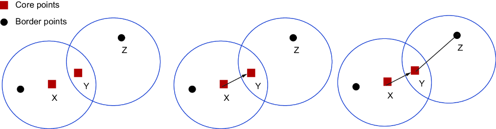
The diagram shows how a point outside one core point’s immediate neighborhood can still be reached through another core point. section 2.5.2

Choosing a radius in Python

On standardized feature data, fit scikit-learn’s NearestNeighbors with n_neighbors=2, sort each observation’s second-neighbor distance, and plot those distances to help choose ε. Then fit DBSCAN with eps as the radius and min_samples as the point threshold; inspect its labels and plot the resulting clusters. The radius is a modeling choice: changing it changes which observations share a neighborhood. section 2.5.2 section 2.5.1

How Data Without Labels covers it

How deep it goes

Defines ε-neighborhood geometry, relates radius to point counts and density, and applies the definition to DBSCAN’s core-point threshold.

Examples

Uses a vector-space circle, connected core points, and Python plots of nearest-neighbor distances and clusters.

What it assumes

Assumes observations can be represented in vector space but defines neighborhoods and their density role from the ground up.

What you can do after

Apply it via scikit-learn’s NearestNeighbors and DBSCAN to inspect radius choices and cluster standardized observations.

How it connects

Connects local neighborhoods to density-based clustering, DBSCAN, core points, outliers and density connectivity.

liveBookmanning.com

Read Data Without Labels on liveBook Get the book at manning.com

Also explained in

• 

  liveBookmanning.com
  Advanced Algorithms and Data StructuresAn epsilon-neighborhood is the set of points within epsilon distance of a specified point.
• 

  liveBookmanning.com
  Graph Neural Networks in ActionA node neighborhood is the set of nodes connected to a particular graph node, typically within a specified number of hops.
• 

  liveBookmanning.com
  Optimization Algorithms: AI techniques for design, planning, and control problemsThe set of candidate solutions reachable from a current solution by permitted local moves.

Compare how 4 books explain local neighborhood →

Related concepts

• graphletused by · A graphlet is a node position within a distinctly connected subgraph consisting of a specified number of nodes.
• graph machine learningused by · Graph machine learning comprises machine-learning methods that learn representations, predictions, or patterns from graph-structured data and relationships.
• pairwise exchangeimplemented by · A pairwise exchange is a neighborhood move that swaps the positions or assignments of two tasks.
• neural message passingused by · Neural message passing is a graph-learning technique that iteratively updates node representations by aggregating information from neighboring nodes.
• data aggregationuses · Data aggregation is the combination of multiple values, records, observations, or results into a consolidated or summarized output.

This explainer was generated by Manning's knowledge graph from the text of Data Without Labels. The section links point to the parts of the book it draws on.