Maximum likelihood estimation (MLE) estimates unknown model parameters by choosing the values that give the greatest likelihood to observed data. It is an estimation framework, not a statistical model: the likelihood depends on the probability model and its assumptions. section 3.1.3 section 3.3
For observed data x and parameter θ, the estimate is θ̂ = arg maxθ L(θ | x). The likelihood L compares parameter values against the same observations; arg max returns the maximizing parameter value, not the likelihood itself. Ronald Fisher formalized this approach in 1922, emphasizing observed data rather than prior distributions. section 3.1.3 section 3.0
Estimating a coin’s probability of heads
If ten tosses yield seven heads, MLE gives p̂ = 7/10 = 0.7 under a model with independent tosses and a constant probability of heads. This is the value most compatible with the sample, not proof that the true probability is exactly 0.7. A larger sample could support a more precise estimate. section 3.1.3 section 10.2.2
To apply MLE, specify a probability model, construct the likelihood for the observations, and maximize it over the unknown parameters. Independent observations allow their individual probabilities or densities to be multiplied. Taking the natural logarithm turns products into sums without changing the maximizing parameter value. Some estimates have analytic solutions; others require numerical optimization. section 3.1.4 section 3.1.5
Estimating a normal mean
For independent observations from a normal distribution with unknown mean μ and known variance, the log-likelihood differs by a constant from −Σ(xᵢ − μ)²/(2σ²). Maximizing it therefore minimizes the sum of squared deviations. Differentiating and setting the derivative to zero gives μ̂ = Σxᵢ/n, the sample mean. section 3.1.4
The same principle connects several modeling methods:
- Logistic regression estimates coefficients from the likelihood of observed binary outcomes, using numerical optimization rather than a closed-form coefficient solution. section 3.3.1 section 3.3.2
- Linear regression with independent, normally distributed errors yields the ordinary least squares coefficient estimates: maximizing likelihood is equivalent to minimizing squared residuals. section 3.4.2
- Neural networks often minimize losses equivalent to negative log-likelihoods: cross-entropy for categorical classification and mean squared error under a normal-error assumption. section 3.5
Figure 3.3 Fitted regression line for the synthetic study-hours data set. Each point represents an observed pair of study hours and exam score, while the line represents the conditional mean estimated by maximum likelihood under the normal-error model. The vertical distance between each point and the line is its residual. Because maximizing the Gaussian likelihood produces the same coefficient estimates as minimizing the sum of squared residuals, this is also the ordinary least squares regression line.
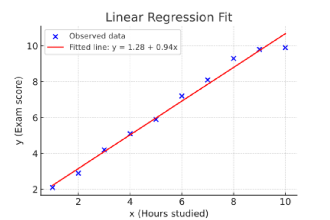
The fitted study-hours regression line shows residuals whose squared sum is minimized by the normal-error maximum likelihood estimates. section 3.4.3
An estimate’s interpretation depends on the assumed model and the available data. Consistency, efficiency, and sufficiency provide standards for evaluating estimators, but maximizing a likelihood alone does not establish that an estimate is exact. MLE also differs from Bayesian updating: it does not assign prior or posterior probabilities to parameter values. section 3.9 section 10.2.2