Gradient descent reduces a loss function by repeatedly moving in the direction of steepest decrease: the negative gradient. In prediction tasks, that loss reflects error between actual and predicted values. In nonmetric multidimensional scaling (MDS), it can be the stress caused by differences between original distances and distances in a lower-dimensional arrangement. section 8.2.6 section 6.2.2
Imagine descending a mountain: at each position, take a step along the steepest downward path, then reassess. A loss function can likewise decrease as its parameters change toward convergence. Convergence does not necessarily establish that the lowest possible value has been found; a local minimum can hide a deeper one elsewhere. section 6.2.2
The variants differ in how much training data contributes before an update:
- Batch gradient descent uses every training instance for an iteration. This can be slow with large or high-dimensional datasets. section 8.2.6
- Stochastic gradient descent (SGD) updates coefficients after each training instance rather than waiting for the full batch. section 8.2.6
- Mini-batch gradient descent uses small subsets to balance speed and accuracy. Batch size becomes a hyperparameter to tune; example sizes include 32, 64, and 128. section 8.2.6
Reducing MDS stress
Suppose points are placed in fewer dimensions. If the distances between their new coordinates are close to their original distances, stress is small. Gradient descent is one way to seek coordinates that reduce this loss; the distance comparison defines the objective, not a guarantee of the global minimum. section 6.2.2
Figure 6.4 While the first figure is the point of convergence and represents the gradient descent method, note that in the second figure the global minima is somewhere else, while the algorithm can be stuck at a local minima. The algorithm might check that it has optimized the cost function and reached the point of global minima, whereas it has only reached the local minima. In a local minima, there is no direction that is ascending; all the directions descend. The algorithm, if purely local, has no information about other deeper minima existing beyond a potentially small hill.
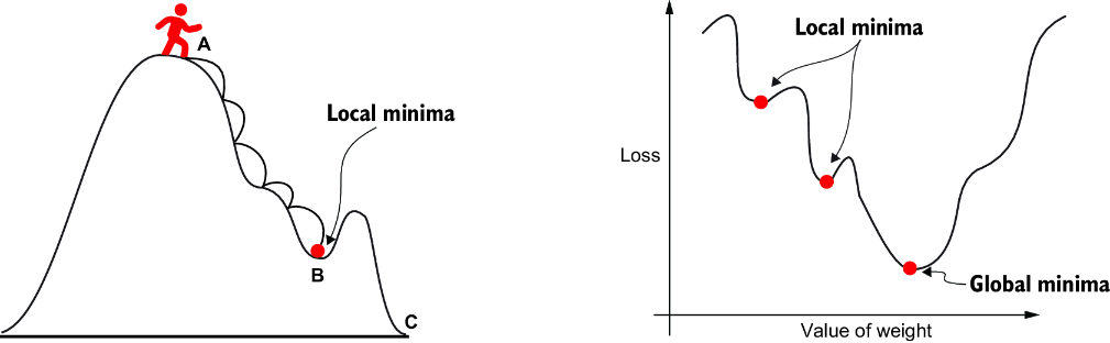
The diagram contrasts convergence with a local minimum, where a locally descending search can miss a lower value elsewhere. section 6.2.2
















