Gradient descent

As explained in Ensemble Methods for Machine Learning

Gradient descent is an iterative optimization method that updates parameters in the direction opposite the loss gradient.

Gradient descent trains a model by treating fit as a minimization problem: define a loss that measures prediction error, then repeatedly change the parameters to lower that loss. Rather than exhaustively testing a parameter grid, it uses first-derivative information to guide the search. section 5.1

The gradient is the local slope of an objective function and points toward steepest ascent. Gradient descent moves in the opposite direction, the negative gradient, so each update heads toward a local minimum. The update combines a direction with a step length, and repeats from an initial parameter guess until the change is sufficiently small. section 5.1.1 section 6.1

Figure 5.2 The surface plot (left) and contour plot (right) of the Branin function. We can visually verify that this function has four minima, which are the centers of the elliptical regions in the contour plot.

Use the surface and contour views to see why following downhill slope can find a minimum, while different starting points can lead to different local minima. section 5.1.1

A practical gradient-descent loop is:

• Start from an initial parameter vector and evaluate the loss gradient there. section 5.1.1
• Negate and normalize the gradient to obtain a downhill direction. section 5.1.1
• Choose a step length with line search, then add the scaled direction to the current parameters. section 5.1.1
• Stop when successive parameter values differ by less than a tolerance; otherwise continue iterating. section 5.1.1

Training a linear classifier

For a noisy, nearly linearly separable two-class data set, a linear classifier is trained from scratch by minimizing vectorized squared loss. Its gradient is computed from the data matrix, labels, and current weights; descent from an initial weight vector learns a separator with reported training accuracy of 0.995. section 5.1.2

Gradient boosting adapts the same idea to sequential ensembles. Direct gradient descent adds the negative gradient to the current model; gradient boosting instead trains a weak regression learner on residuals, which approximate that negative gradient. Its step length corresponds to the weight assigned to each base estimator. section 5.2.1

Figure 5.9 Comparing gradient descent (left) to gradient boosting (right). At iteration t, gradient descent updates the model using the negative gradient, -g_t. At iteration t, gradient boosting approximates the negative gradient by training a weak regressor, h_t, on the negative residuals -r^t_i. The step length α_t in gradient descent is equivalent to the hypothesis weight of each base estimator in a sequential ensemble.

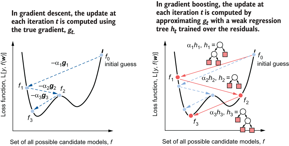
Compare the direct negative-gradient update with the weak-regressor approximation used by gradient boosting. section 5.2.1

Step length matters because first-order information produces only a local linear approximation. Newton’s method contrasts with gradient descent by also using second-derivative information, forming a local quadratic approximation that can yield better steps and faster convergence. section 6.1

How Ensemble Methods for Machine Learning covers it

How deep it goes

Works through negative-gradient updates, normalization, line search, tolerance, and vectorized squared-loss training; defers numerical gradient alternatives.

Examples

Uses Branin-function contour descent and a noisy two-class linear classification task with squared loss.

What it assumes

Reinforces loss functions, predicted versus true labels, parameters, and first derivatives before applying updates.

What you can do after

Build it from scratch for a differentiable objective and apply it to train a simple linear classifier.

How it connects

Connects loss functions, residuals, AdaBoost, gradient boosting, regression trees, and Newton’s method.

liveBookmanning.com

Read Ensemble Methods for Machine Learning on liveBook Get the book at manning.com

Also explained in

• 

  liveBookmanning.com
  Advanced Algorithms and Data StructuresGradient descent is an iterative optimization technique that moves a candidate solution in the direction of decreasing objective-function value using gradient information.
• 

  liveBookmanning.com
  Grokking Machine LearningAn iterative optimization technique that changes parameters in the direction of greatest local decrease of an objective function.
• 

  liveBookmanning.com
  Deep Learning with R, Third EditionGradient descent is an iterative optimization algorithm that updates parameters in the direction opposite to a function's gradient to reduce a loss or objective.
• 

  liveBookmanning.com
  Deep Learning with PyTorch, Second Edition
• 

  liveBookmanning.com
  Deep Learning with JAXAn optimization step that updates model parameters using gradients, typically in the opposite direction of the loss gradient.
• 

  liveBookmanning.com
  Machine Learning for Tabular Data: XGBoost, Deep Learning, and AIGradient descent is an optimization technique that iteratively adjusts parameters in the direction that reduces a differentiable objective function.
• 

  liveBookmanning.com
  Sutskever's ListGradient descent is an iterative optimization method that changes parameters in the direction opposite the gradient of a loss function.
• 

  liveBookmanning.com
  Deep Learning with Python, Third EditionA parameter update step computed from gradients to reduce model error.
• 

  liveBookmanning.com
  Data Without LabelsGradient descent is an iterative optimization technique that updates parameters in the direction of decreasing objective-function value.
• 

  liveBookmanning.com
  Math and Architectures of Deep Learning
• 

  liveBookmanning.com
  Grokking AI Algorithms, Second EditionGradient descent is an optimization technique that iteratively changes parameters in the direction that reduces an objective function.
• 

  liveBookmanning.com
  How Large Language Models WorkGradient descent is an iterative optimization algorithm that adjusts parameters in the direction that reduces a differentiable objective function.
• 

  liveBookmanning.com
  Classic Computer Science Problems in Swift: Essential techniques for practicing programmers
• 

  liveBookmanning.com
  Reinforcement Learning from Human FeedbackA gradient update, or gradient step, changes model parameters using the gradient of an optimization objective.
• 

  liveBookmanning.com
  Bayesian Optimization in ActionGradient descent is an iterative optimization technique that updates parameters in the direction opposite the objective gradient.
• 

  liveBookmanning.com
  Optimization Algorithms: AI techniques for design, planning, and control problemsAn iterative optimization algorithm that changes variables in the direction of the negative gradient to reduce a differentiable objective function.

Compare how 17 books explain gradient descent →

Related concepts

• gradientuses · A gradient is the vector of partial derivatives of a scalar function with respect to its variables, indicating its local rate and direction of change.
• stochastic gradient descentincludes · Stochastic gradient descent is an iterative optimization method that updates parameters using gradients estimated from individual examples or randomly selected small batches.
• parameteruses · A model parameter is a numerical value, such as a weight or bias, that is learned or set to determine how a model computes outputs.
• neural networkused by · A neural network is a computational model of interconnected, parameterized units that learns transformations from inputs to outputs.
• regularizationuses · Regularization is a modeling technique that constrains or penalizes solutions during fitting or optimization to discourage undesirable complexity or behavior and improve generalization or estimation.
• newton-raphson methodcontrasts with · The Newton-Raphson method is an iterative numerical technique that uses first- and second-derivative information to find a root or optimize an objective.

This explainer was generated by Manning's knowledge graph from the text of Ensemble Methods for Machine Learning. The section links point to the parts of the book it draws on.