Imagine standing on Mount Errorest in fog: to reduce a model’s error, take a small step in the direction that descends most, then repeat. Gradient descent changes model parameters iteratively toward lower error. section 3.4
Figure 3.20 We are on top of Mount Errorest and wish to get to the bottom, but we can’t see very far. A way to go down is to look at all the directions in which we can take one step and figure out which one helps us descend the most. Then we are one step closer to the bottom.
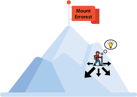
Use the mountain analogy to visualize choosing a locally descending direction when the full error landscape is not visible. section 3.4
A practical gradient-descent cycle looks like this:
- Start with a model and measure its error using an error function such as absolute error or square error. section 3.4
- Use the gradient to identify the direction that decreases the error most locally. section 3.4
- Take a small parameter step, with the learning rate controlling the update size, and repeat. section 5.3 section 3.4
- Track the error while iterating and stop when additional iterations no longer provide useful improvement. section 3.4
From a line to a classifier
For linear regression, gradient descent reduces an error function measuring distances between data points and a line. In a perceptron example, a misclassified sentence changes its word weights and bias: with learning rate 0.01, weights 1 and 2 become 0.98 and 1.95, while bias −4 becomes −4.01, lowering the example’s error from 8 to 7.7. section 3.4 section 5.3
Figure 3.23 The plot of the root mean square error for our running example. Notice how the algorithm succeeded in reducing this error after a little over 1,000 iterations. This means that we don’t need to keep running this algorithm for 10,000 iterations, because around 2,000 of them do the job.
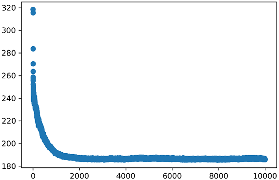
The error plot shows why monitoring iterations matters: the running example reduces root mean square error after slightly more than 1,000 iterations. section 3.4
















