Gradient descent is an optimization procedure for reducing a model’s error. It begins with an initial set of model weights, measures error, computes the gradient with respect to those weights, and adjusts them repeatedly in the direction that lowers error. The mountain-descent analogy is useful: the error surface is the landscape, and the goal is to reach a low valley rather than remain high on the surface. section 4.3.5
Figure 4.12 Gradient descent optimization in action in a simple optimization landscape
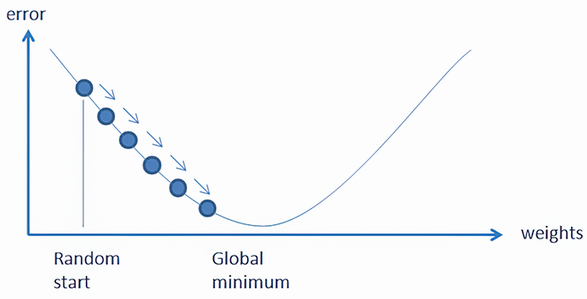
Visualize successive weight updates as a descent from a random starting point toward the minimum of a bowl-shaped error curve. section 4.3.5
The update path matters. Complex error landscapes can contain local minima and plateaus, so iterative adjustment need not produce the best possible solution. Gradient descent nevertheless supplies the core optimization idea behind linear models, stochastic learning, and deep learning. section 4.3.5
Two practical uses illustrate how the procedure changes with the modeling workflow:
- Stochastic gradient descent (SGD) updates linear-model weights from small batches or individual streamed examples. This makes out-of-core learning possible when data cannot be retained for repeated full-dataset passes; reserve a test set when cross-validation is impractical. section 4.3.5
- Gradient boosting adds decision trees sequentially, with each tree correcting errors from the preceding ensemble. The process resembles gradient descent over the combined model’s error, while each individual tree also has its own optimization. section 5.2
Boosted classification with a learning rate
For binary classification, a gradient-boosting implementation can start from the target’s average probability, convert it to a logit, calculate gradients from predicted and actual values, then fit regression trees as successive corrections. The learning rate controls the size of those corrections, while the number of estimators controls how many trees are added. section 5.2.1
For tabular prediction, gradient boosting combines gradient-based correction with decision trees. It can capture nonlinear relationships, requires no feature scaling or monotone transformation, and can handle missing data, noisy observations, and outliers; performance still depends on hyperparameter tuning. section 5.2 section 5.6
Listing 4.10 Out-of-core logistic regression with L2 regularization
from sklearn.linear_model import SGDClassifier
from sklearn.model_selection import train_test_split
from sklearn.utils import gen_batches
from sklearn.metrics import accuracy_score

def generate_batches(X,
                     y,
                     batch_size,
                     random_state):                                 #1
    """split dataset into batches """
    examples = len(X)
    batches = gen_batches(n=examples,
                          batch_size=batch_size)                    #2
    sequence = np.arange(examples)
    if random_state:
        np.random.seed(random_state)                                #3
        np.random.shuffle(sequence)

    for batch in batches:
        items = sequence[batch]
        yield(X.iloc[items], y.iloc[items])                         #4

model = SGDClassifier(loss="log_loss",
                      average=True,
                      penalty='l2',
                      alpha=0.001)                                  #5

column_transform = ColumnTransformer(
    [('categories', categorical_onehot_encoding, low_card_categorical),
     ('numeric', numeric_standardization, continuous)],
    remainder='drop',
    verbose_feature_names_out=False,
    sparse_threshold=0.0)

X_train, X_test, y_train, y_test = train_test_split(data, target_median,
                                                    test_size=0.20,
                                                    random_state=0) #6
iterations = 10
for j in range(iterations):                                         #7
    generator = generate_batches(X_train, y_train, batch_size=256,
random_state=j)
    for k, (Xt, yt) in enumerate(generator):
        if k == 0:
            column_transform.fit(Xt)
                    Xt = column_transform.transform(Xt)
        if k == 0:
            model.partial_fit(Xt, yt, classes=(0, 1))               #8
        else:
            model.partial_fit(Xt, yt)                               #9

predictions = model.predict(column_transform.transform(X_test))
score = accuracy_score(y_true=y_test, y_pred=predictions)
print(f"Accuracy on test set: {score:0.3f}")                        #10
Inspect an out-of-core logistic-regression workflow that shuffles data, yields batches, trains an SGD classifier, and evaluates reserved test data. section 4.3.5
















