Monte Carlo simulation estimates a quantity by generating random samples and averaging values calculated from them. In Bayesian inference, samples can stand in for a posterior distribution when no closed-form solution is available, especially with non-conjugate priors. section 5.3 section 5.0
Samples provide practical approximations for several distributional quantities:
- Estimate a mean with the average of the samples. section 5.3
- Estimate a credible interval with sample quantiles, such as the 2.5th and 97.5th percentiles for a 95% interval. section 5.3
- Estimate a tail probability or CDF value with the proportion of samples below a threshold. section 5.3
- Use MCMC when independent samples are unavailable; diagnose chains with burn-in removal, multiple initializations, R̂, ESS, and trace plots. section 5.14
Choosing whether to launch a design
Draw 100,000 samples of the uncertain conversion rate, calculate the launch utility for each sample, and average those utilities. The estimated launch utility is about $107,496, compared with $100,000 for not launching, so the launch decision is preferred. section 12.5
Figure 5.1 Comparison between a posterior distribution available in closed form and Monte Carlo samples. The samples’ histogram matches the true PDF, and the various statistics from the samples give reasonable approximations to the corresponding true quantities.
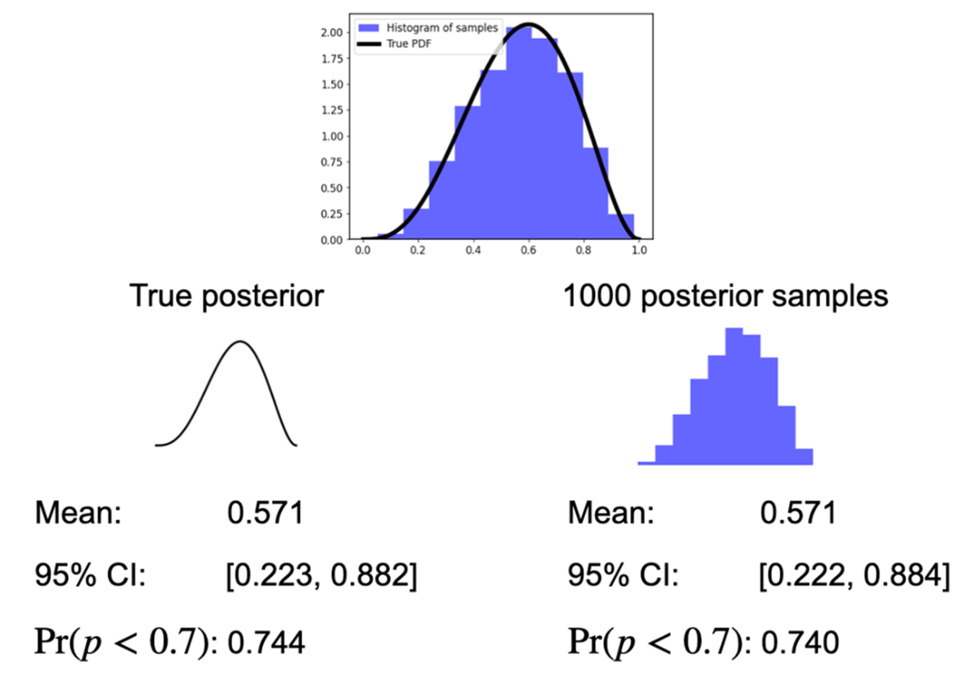
Compare a true posterior with a histogram of Monte Carlo samples and see how sample-based statistics approximate the underlying distribution. section 5.3