Suppose a nearest-neighbor search must find points near a given location. A regular grid divides the coordinate space into equal-sized cells, like tiles on a map. Dividing each coordinate by the corresponding cell size identifies the cell containing a point. The search can then examine points in that cell and neighboring cells instead of starting with every point. section 8.2.2
That shortcut depends on how points are distributed. When data forms dense clusters separated by sparse areas, many cells may be empty while a few hold hundreds or thousands of points. Those crowded cells still require many comparisons. A regular grid is therefore easy to index, but it is not necessarily a good nearest-neighbor index for irregular data. section 8.2.2
The same partition can organize parallel DBSCAN work:
- Split each coordinate’s domain into cells. A cell is a rectangle in two dimensions or a hyper-rectangle in higher dimensions; side lengths may differ across coordinates. section 13.4
- Extend each cell by ε in every direction to form an overlapping shard. This places a point’s ε-neighborhood inside at least one shard when the point lies near a shared border. section 13.4
- Run DBSCAN on the shards, then merge clusters across adjacent shards using their shared margin points. Overlap preserves border relationships but causes some points to be processed more than once. section 13.4
Figure 13.12 Sharding data for MapReduce DBSCAN (MR-DBSCAN). After dividing the domain into equally sized cells, for each shard we need to include all points in one cell, plus all the points within a distance equal to ϵ from its borders. In practice, instead of the cells, we take a rectangle obtained by stretching the cell further in all directions, and each of the sides will measure like the corresponding cell’s side plus 2ϵ. This way, core points close to the cells’ borders will have their ϵ-neighborhood contained in either shard.
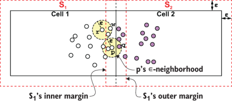
The diagram shows why a DBSCAN shard includes its cell plus an ε-wide margin: a core point near a border can retain its neighborhood within an extended cell. section 13.4
Grid lookup and border checks are simple: border proximity can be tested coordinate by coordinate rather than by measuring distance to a spherical canopy. The trade-off is workload balance. Sparse and crowded cells limit the savings in nearest-neighbor search, while overlapping shards duplicate some clustering work. The useful question is not just whether cells are cheap to locate, but whether their point counts and margins make the partition worthwhile. section 8.2.2 section 13.4