Regression discontinuity design

As explained in Causal Inference for Data Science

Regression discontinuity design is a causal estimation method that exploits an abrupt change in treatment assignment or exposure at a time or threshold cutoff.

Regression discontinuity design (RDD) estimates a causal effect when treatment or exposure changes abruptly at a known time or cutoff. It is useful when an A/B test is impractical: for example, a streaming service cannot release a popular film only to selected customers, but can examine whether views of an older film jump when the new film launches. section 11.0 section 11.2

A simple before-and-after comparison can confuse the event with seasonality or other simultaneous influences. RDD instead focuses on observations close to the event: if competing influences change gradually, they should affect outcomes similarly immediately before and after the cutoff. The remaining discontinuity estimates the event’s causal effect under this local-randomization assumption. section 11.2

Apply the design by:

• Identifying the event date or assignment threshold and measuring the outcome on both sides. section 11.2
• Restricting attention to a small interval around the cutoff, where gradual influences are approximately balanced. section 11.2
• Estimating the jump at the cutoff rather than attributing every before-after difference to the event. section 11.2
• Checking practical approaches such as differences in means or linear regression without ignoring their limitations. section 11.5

A movie-release discontinuity

Suppose daily views of Revenge of the Sith follow a trend but spike when The Force Awakens is released. Compare observations immediately before and after the release, treating slowly changing influences as locally equivalent. Synthetic data with a spike and subsequent decline can test whether the estimation procedure behaves correctly. section 11.0 section 11.2

Figure 11.2 Data simulating the number of views of III. There is a spike in views, followed by a decreasing trend. We can check whether our algorithms are working correctly by testing them on simulated data.

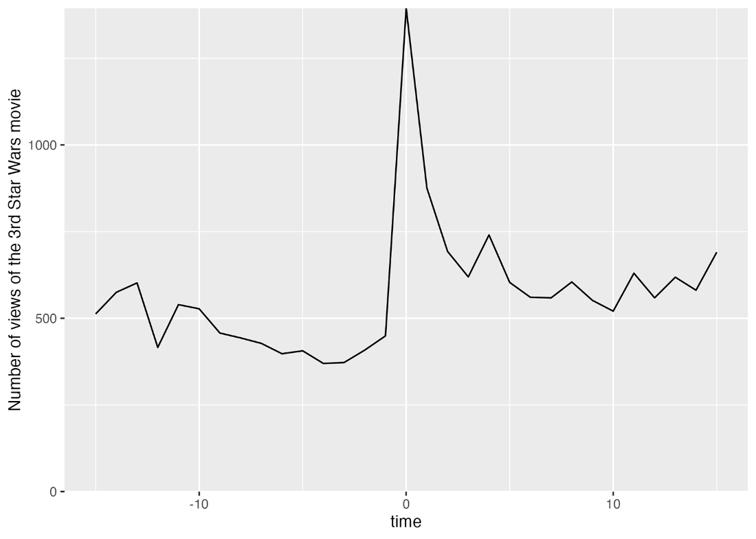
Inspect the simulated time series to see the cutoff-related spike and the following decline before considering an estimated effect. section 11.2

How Causal Inference for Data Science covers it

How deep it goes

Explains local randomization intuitively, demonstrates near-cutoff estimation, and flags limitations of common fitting approaches.

Examples

Uses a Star Wars movie release, Google Trends interest, and simulated daily viewership with a cutoff spike.

What it assumes

Assumes recognition that gradual influences differ less between observations near an event than across distant dates.

What you can do after

Estimate an average treatment effect from time-series observations surrounding an event cutoff.

How it connects

Connects causal estimation with A/B testing, time series data, synthetic controls, and differences-in-differences.

liveBookmanning.com

Read Causal Inference for Data Science on liveBook Get the book at manning.com

Related concepts

• linear regressionused by · Linear regression is a statistical modeling method that estimates a continuous response as a linear combination of predictor variables and fitted coefficients.
• mean differenceused by · A mean difference is a statistic calculated by subtracting the arithmetic mean of one group or condition from that of another.
• treatment effectproduces · A treatment effect is the difference in an outcome attributable to receiving an intervention or exposure rather than a comparison condition.
• local linear regressionuses · Local linear regression estimates a locally linear relationship by fitting weighted linear models around each prediction point.

This explainer was generated by Manning's knowledge graph from the text of Causal Inference for Data Science. The section links point to the parts of the book it draws on.