Root mean squared error

As explained in Demand Forecasting Best Practices

Root mean squared error is the square root of the mean of the squared differences between forecast values and corresponding actual values.

RMSE measures forecast accuracy by taking the square root of the average squared differences between forecast and actual demand. Its squared-error weighting gives large mistakes more influence than small ones, making it useful when major forecast errors create disproportionate supply-chain consequences such as lost sales or dead stock. section 8.5 section 8.5.3

Four-period demand example

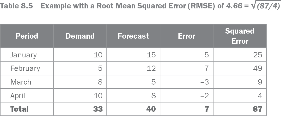
For January through April, the squared errors are 25, 49, 9, and 4, totaling 87. RMSE = √(87/4) = 4.66. The result is an absolute measure in demand units, not a percentage. section 8.5 section 8.5.1

Use RMSE deliberately when comparing forecasts:

• Prefer it when the largest errors deserve extra attention or when evaluating safety-stock-related accuracy. section 8.5.3
• Avoid treating it as universally best: outliers and highly variable demand can make RMSE overreact to a few periods. section 9.1
• Use caution across product portfolios, where squaring errors overemphasizes high-volume items; RMSE is better suited to a single product. section 11.2
• Pair accuracy with bias rather than selecting a forecast from RMSE alone; a combined MAE and absolute-bias score can provide a more robust compromise. section 9.4 section 9.3

Table 8.5 Example with a Root Mean Squared Error (RMSE) of 4.66 = √(87/4) (view table figure)

Period	Demand	Forecast	Error	Squared Error
January	10	15	5	25
February	5	12	7	49
March	8	5	–3	9
April	10	8	–2	4
Total	33	40	7	87

Inspect the period-by-period demand, forecast, error, and squared-error table behind the 4.66 calculation. section 8.5

Figure 8.10 How to compute the root mean squared error (RMSE) in Excel

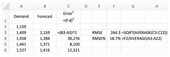
Follow the spreadsheet layout for calculating squared errors and the final RMSE in Excel. section 8.5.2

How Demand Forecasting Best Practices covers it

How deep it goes

Defines the formula, works a four-period calculation, illustrates Excel steps, and explains weighting, outliers, bias, and portfolio limits.

Examples

Uses a four-period demand table, Excel calculations, an intermittent-demand comparison, and a product-portfolio example.

What it assumes

Assumes actual demand and forecast values, while teaching squared errors, averaging, square roots, and percentage scaling.

What you can do after

Apply it via Excel to calculate forecast error, compare forecasts, and judge when large errors should dominate evaluation.

How it connects

Connects forecast error, MAE, MAPE, bias, safety stock, intermittent demand, outliers, and inventory optimization.

liveBookmanning.com

Read Demand Forecasting Best Practices on liveBook Get the book at manning.com

Also explained in

• 

  liveBookmanning.com
  Grokking Machine LearningA regression metric equal to the square root of the average squared difference between observed and predicted target values.
• 

  liveBookmanning.com
  Starting Data Analytics with Generative AI and PythonRoot mean squared error is the square root of mean squared error and expresses prediction error in the dependent variable's units.
• 

  liveBookmanning.com
  Effective Data AnalysisRoot mean squared error is the square root of the mean squared differences between predicted and actual numerical values.
• 

  liveBookmanning.com
  Machine Learning for Tabular Data: XGBoost, Deep Learning, and AIRoot mean squared error is the square root of the mean squared differences between predicted and observed numeric values.
• 

  liveBookmanning.com
  Investing for ProgrammersRoot mean-squared error is the square root of the average squared difference between predicted and observed values.
• 

  liveBookmanning.com
  AI-Powered SearchRoot mean square error is the square root of the mean squared difference between predicted and actual values.

Compare how 7 books explain root mean squared error →

Related concepts

• mean squared erroruses · Mean squared error is the arithmetic mean of the squared differences between corresponding predicted and target numerical values.
• forecast erroruses · A forecast error is the difference between an observed value and the corresponding forecasted value.
• linear regressionmeasures · Linear regression is a statistical modeling method that estimates a continuous response as a linear combination of predictor variables and fitted coefficients.
• language modelmeasures · A language model is a computational model that represents patterns in linguistic tokens to estimate sequence probabilities and predict or generate language from context.
• objective functionkind of · An objective function assigns values to candidate solutions, predictions, or parameter settings according to a criterion to be minimized or maximized.
• squared lossused by · Squared loss is the square of the difference between a predicted or fitted value and its target or observation, often summed across data points.

This explainer was generated by Manning's knowledge graph from the text of Demand Forecasting Best Practices. The section links point to the parts of the book it draws on.