A search space is the set of candidate points, states, or solutions that an algorithm can inspect and transform. Its structure determines which search operations are useful: an ordered one-dimensional space supports left-right partitioning, while higher-dimensional spaces require partitions that preserve more than one coordinate. section 8.2.3 section 8.4.2
Reason about a search space by identifying:
- Its representation: a line of ordered real numbers, a geometric domain, or a collection of discrete arrangements. section 8.4.1 section 17.2.2
- Its partitioning rule: binary search can repeatedly halve an ordered line, but a plane cannot be divided reliably by considering only one coordinate. section 8.4.1 section 8.4.2
- Its transitions: optimization methods move between candidate solutions, balancing nearby refinement against distant moves that can escape local minima. section 17.1.4
- Its size and cost: exhaustive evaluation may work for a small space but become impractical as the number of candidates grows. section 17.2.2
From warehouse locations to route permutations
For nearest-neighbor search, cities, warehouses, and customers can be projected onto a one-dimensional road. The ordered coordinates allow binary search to narrow the candidates and compare the remaining closest points. For the traveling salesperson problem, the search space instead contains every permutation of the vertices; six cities produce 720 candidates, while larger graphs quickly make exhaustive search impractical. section 8.2.3 section 17.2.2
Figure 17.9 The cost landscape for the TSP applied to the graph in figure 17.8 (A). The cost function is displayed for the whole domain; it’s hard to make sense of it! 17.8 (B) Zooming in on the first few hundreds of permutations, we can see that there are several local minima.
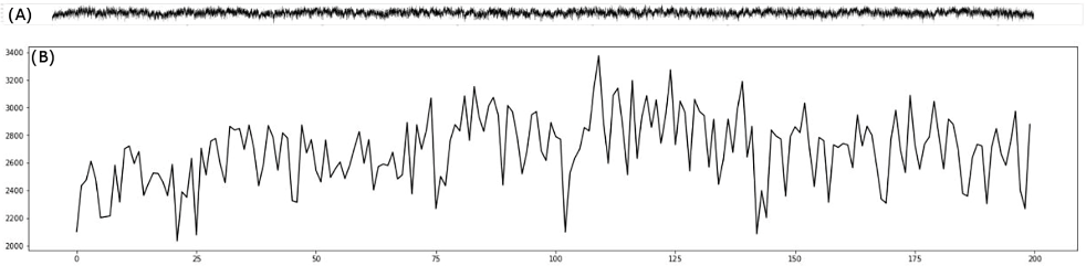
Inspect the cost landscape to see how a large search space contains local minima and why optimization may examine only part of it. section 17.2.2