Suppose 20 runs produce timings from 0.1 to 1.3 seconds, with a mean of 0.6 seconds. The range and standard deviation describe variation; skew describes whether the timings are lopsided around the mean. Do not infer skew from the endpoints alone: inspect how often values occur on each side. section 16.4
Figure 16.1 Frequency histogram for our sample, showing the frequency with which each of the measured values was obtained
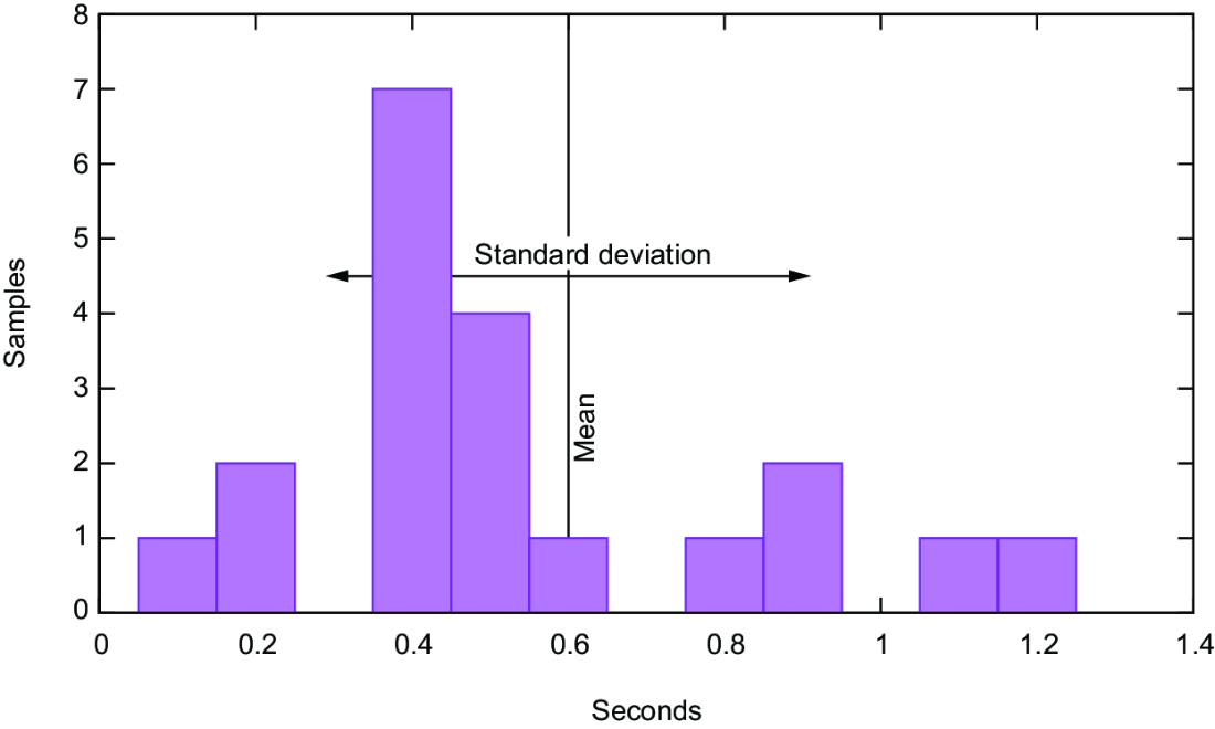
The frequency histogram shows how often each of the 20 timings occurred, making the distribution easier to inspect than a list of values. section 16.4
TAKEAWAY: Repeated timings need more than an average when measurements vary substantially. Skew can help characterize their asymmetry, but collecting statistics also changes the measurement. In the illustrated comparison, adding skew collection increased measured time per iteration by 9% over the preceding setup. section 16.4
Table 16.1 Comparison of measurements
| Loop | Sec per iteration | Difference | Gain/loss | Conclusive | |
|---|---|---|---|---|---|
| 0 | volatile loop |
1.97⋅10-09 | |||
| 1 | volatile store |
3.66⋅10-10 | -1.60⋅10-09 | -81% | Yes |
| 2 | Opaque addition | 3.45⋅10-10 | -2.10⋅10-11 | -6% | No |
| 3 | Plus timespec_get |
1.77⋅10-08 | 1.74⋅10-08 | +5043% | Yes |
| 4 | Plus mean | 2.62⋅10-08 | 8.5⋅10-09 | +48% | Yes |
| 5 | Plus variance | 2.90⋅10-08 | 2.8⋅10-09 | +11% | Yes |
| 6 | Plus skew | 3.17⋅10-08 | 2.7⋅10-09 | +9% | Yes |
The comparison table separates the cost of collecting skew from earlier additions of the mean and variance. section 16.4