Surrogate model

As explained in Experimentation for Engineers

A surrogate function is a model that approximates a measured response as a function of parameter values and estimates the response at unmeasured values.

A surrogate model approximates a measured response as a function of one or more parameter values. It interpolates from aggregate experimental measurements to estimate a business metric at settings that have not been measured. Those estimates are cheap to generate—milliseconds rather than the hours or weeks an experiment may require—so they support searching for promising settings before committing to more production measurement. section 4.1 section 4.3

In response surface methodology, the target being approximated is the response surface: the underlying relationship between parameters and a metric such as profit. For a continuously varying metric over a continuous parameter, measured values can be interpolated between. Domain knowledge should first constrain the parameter range to settings where the system can function, and the experiment must include enough useful measurement locations for the analysis. section 4.1.1 section 4.1.3

One-parameter profit model

A trading strategy uses a signal threshold to decide when to buy or sell. After measuring aggregate markout profit at three threshold values, fit a quadratic surrogate with linear regression: profit is modeled as a constant, a linear threshold term, and a squared threshold term. Evaluate the fitted parabola across a fine grid of thresholds, then select the threshold with the largest estimated profit. With exactly three aggregate measurements and three fitted coefficients, the curve fits those measurements exactly; with additional measurements, approximation error is expected. section 4.1.1 section 4.1.3

Use a surrogate model as an iterative experimental decision tool:

• Choose feasible parameter values using engineering or business knowledge and the needs of the planned analysis. section 4.1.1
• Measure the business metric at the selected settings and aggregate the individual results. section 4.1
• Fit the surrogate, search it for an estimated optimum, and redesign the experiment if analysis does not locate one. section 4.1
• Validate the selected setting experimentally; return to design when the observed result does not agree with the estimate. section 4.1 section 4.3

For two parameters, a quadratic surrogate expands to include a linear and squared term for each parameter plus a cross term. The cross term represents behavior along diagonal regions between design points. A fitted two-dimensional surface can provide many estimates from relatively few measurements, but its complexity raises the need to inspect the experiment: an outlying measurement can violate the assumption that the model is being fit near an optimum, prompting another iteration. section 4.2.2 section 4.2.2

Figure 4.18 A two-dimensional surrogate function, an interpolation of markout_profit_2D over settings of threshold and order_size. The filled dots mark the parameter settings where markout profit was measured in the experiment. In this figure, there are many more estimates of markout profit (around 20,000 interpolation estimates) than measurements (only nine).

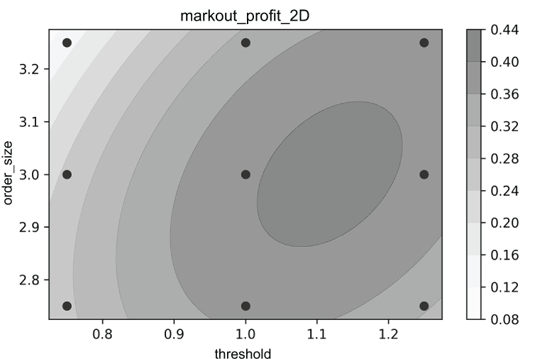
Inspect the fitted surface as a grid of estimates over threshold and order size, with measured settings marked separately from interpolated values. section 4.2.2

A surrogate can also guide which experiment to run next. In Bayesian optimization, it models CPU time versus a parameter from sparse evidence while representing uncertainty: a single measurement can anchor the estimated response at its observed value, with uncertainty assumed to grow away from that point under a continuity assumption. section 6.1.3

How Experimentation for Engineers covers it

How deep it goes

Works through one- and two-parameter quadratic regressions, interpolation grids, optimization, iteration, and validation.

Examples

Uses simulated trading markout profit over threshold and order size, plus CPU time from one Bayesian-optimization measurement.

What it assumes

Assumes aggregate experimental measurements and continuous feasible parameter ranges; defers linear-regression introduction to an appendix.

What you can do after

Apply it via linear regression to estimate and optimize parameter settings, then validate the estimated optimum experimentally.

How it connects

Connects response surface methodology with interpolation, linear regression, Bayesian optimization, continuous parameters, and validation.

liveBookmanning.com

Read Experimentation for Engineers on liveBook Get the book at manning.com

Also explained in

• 

  liveBookmanning.com
  Bayesian Optimization in ActionA surrogate model is a predictive model that approximates an objective function from observed evaluations.
• 

  liveBookmanning.com
  Outlier Detection in PythonA proxy model is an approximate model that imitates the behavior of another model or detector for analysis or explanation.
• 

  liveBookmanning.com
  Ensemble Methods for Machine LearningA surrogate model is an interpretable approximation trained to reproduce the behavior of a more complex model in a specified region or representation.
• 

  liveBookmanning.com
  Machine Learning for Tabular Data: XGBoost, Deep Learning, and AIA surrogate function is an approximate model of an objective function that predicts objective behavior across untested parameter settings.

Compare how 5 books explain surrogate model →

Related concepts

• Optunaused by · Optuna is an open-source Python framework for automated hyperparameter optimization through repeated trials that explore parameter configurations.
• Bayesian optimizationused by · Bayesian optimization is a sequential method for optimizing an expensive or unknown objective by using a probabilistic model to guide evaluations.
• interpretabilityused by · Interpretability is the degree to which people can understand a model’s behavior, outputs, predictions, or the factors that produce them.
• black boxuses · A black box is a system or component whose internal workings are treated as opaque while its inputs, outputs, or observable behavior are considered.
• Gaussian processproduced by · A Gaussian process is a probability distribution over functions in which every finite collection of function values has a joint Gaussian distribution.
• labelcontrasts with · A label is a value or annotation associated with an item that identifies its target category, outcome, or reference answer for learning or evaluation.

This explainer was generated by Manning's knowledge graph from the text of Experimentation for Engineers. The section links point to the parts of the book it draws on.