Network topology

As explained in Deep Learning with R, Third Edition

Network topology is the structural arrangement and connectivity pattern of a neural network's layers and operations.

Network topology is the pattern of connections between a model’s layers and operations. A simple topology stacks layers from one input to one output. Others branch, combine paths, or use residual connections. In Keras, these arrangements form a graph of layers represented by a Model. section 3.6.3

Start with a stack

For vector data, a straightforward topology passes the input through two Dense layers and then a single-unit output layer: inputs <- keras_input(shape = c(num_input_features)) outputs <- inputs |> layer_dense(32, activation = "relu") |> layer_dense(32, activation = "relu") |> layer_dense(1, activation = "sigmoid") model <- keras_model(inputs, outputs) model |> compile(optimizer = "rmsprop", loss = "binary_crossentropy") This configuration is for binary classification. The connections form a stack; the final activation and loss match the task. section 20.1.6

Topology is a consequential choice, not just a drawing. It defines the series of tensor operations through which inputs become outputs, restricting the functions the model’s weights can represent—its hypothesis space. A single Dense layer without an activation, for example, assumes that two classes are linearly separable. Convolution layers instead encode an assumption about patterns in images: their relevance does not depend on location. section 3.6.3 section 9.0

Useful patterns go beyond a plain stack:

• Branches and multiple heads connect layers along more than one path; residual connections are another common topology. section 3.6.3
• Convnet blocks reuse groups of layers. Feature hierarchies can grow deeper in filters while shrinking in spatial size; residual connections address a limit on stacking layers caused by vanishing gradients. section 9.1
• Architecture families suit different data structures: Dense networks commonly handle vectors, convnets images, and recurrent networks or Transformers timeseries. section 20.1.6

Figure 9.2 The “entry flow” of the Xception architecture: note the repeated layer blocks and the gradually shrinking and deepening feature maps, going from 299 × 299 × 3 to 19 × 19 × 728

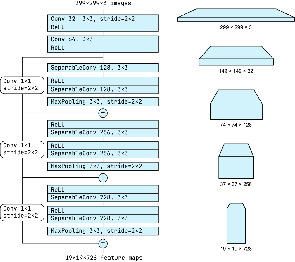
Trace the repeated layer blocks and the changing feature-map sizes in an Xception convnet. section 9.1

Choose an architecture whose assumptions fit the data, then test it against a simple baseline. Once the model can overfit, try adding or removing layers and evaluate each revision on validation data. Reusing validation feedback too many times can itself lead to overfitting; reserve the test set for a final evaluation. In Keras, Sequential handles simple stacks, while the Functional API or Model subclassing can express more involved graphs. section 6.2.3 section 6.2.5 section 3.6.3

How Deep Learning with R, Third Edition covers it

How deep it goes

Explains topology through stacks, branches, feature hierarchies, and architecture assumptions; defers detailed construction of nonsequential models.

Examples

Uses an R/Keras Dense classifier, a Transformer layer graph, and repeated Xception convnet blocks.

What it assumes

Starts from simple Sequential stacks and introduces graphs of layers before more involved topology construction.

What you can do after

Evaluate/understand whether an architecture’s connections and assumptions suit the data, then tune layers using validation results.

How it connects

Links topology to hypothesis spaces, gradient descent, residual connections, feature hierarchies, and data modalities.

liveBookmanning.com

Read Deep Learning with R, Third Edition on liveBook Get the book at manning.com

Also explained in

• 

  liveBookmanning.com
  Secure APIsNetwork topology is the arrangement and connectivity relationships among networks, hosts, and communication components.
• 

  liveBookmanning.com
  Kafka for ArchitectsA graph topology is a directed processing structure that defines how streaming records traverse processing steps.

Compare how 3 books explain network topology →

Related concepts

• directed acyclic graphkind of · A directed acyclic graph is a graph with directed edges and no directed cycles.
• full mesh topologyincludes · A full mesh topology is a network arrangement in which every node has a direct connection to every other node.
• TensorBoardused by · TensorBoard is a web-based tool for visualizing and monitoring machine-learning experiments and their logged data, including metrics, model graphs, and other run information.
• hypothesis spaceconfigures · A hypothesis space is a set of candidate functions, models, parameter configurations, or rules that a learning or inference procedure can represent or consider.
• star topologyincludes · A star topology is a network arrangement in which multiple peripheral nodes connect and communicate through a central hub or node.

This explainer was generated by Manning's knowledge graph from the text of Deep Learning with R, Third Edition. The section links point to the parts of the book it draws on.