A neural network is a prediction function built from connected layers. Each layer applies a linear transformation followed by a nonlinear activation function, allowing many layers to represent complex mappings from inputs to outputs. section 10.1
Understand a neural network through its parts:
- Nodes represent dimensions within a layer, while edges connect successive layers. section 10.1
- Edge weights provide the coefficients of each linear transformation, and biases provide the additional offset in y = mx + b. section 10.1
- Input and output dimensions follow the learning problem; intermediate hidden-layer sizes are design choices. section 10.1
- A standard network produces a prediction from parameters, commonly written as f(x; w), but does not inherently quantify prediction uncertainty. section 10.1
Learning a noisy curve
A network can be trained on one-dimensional data generated from a sine function and corrupted by noise, then used to predict across a wider input range. Its architecture and learned weights determine the resulting curve, while a standard network’s predictions do not show uncertainty from observation noise or sparse data. section 10.1
Figure 10.2 The architecture of an example neural network with two hidden layers of size 6 and 4.
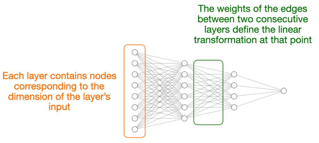
Inspect a two-hidden-layer architecture with hidden layers of sizes 6 and 4 to see how nodes, edges, weights, and biases form a network. section 10.1
Figure 10.3 Predictions made by a standard neural network, which don’t include uncertainty quantification despite its importance in indicating both observation noise and data sparsity.
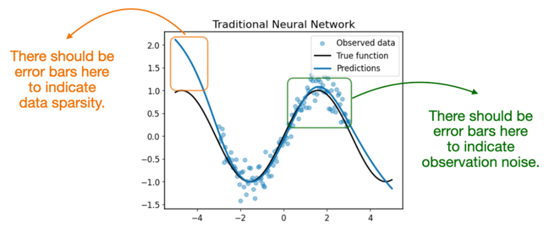
Compare standard neural-network predictions with the uncertainty information needed to indicate observation noise and sparse data. section 10.1