A binomial distribution models the number of successes in a fixed number of repeatable trials. Each trial has two outcomes, success or failure, and shares the same success probability. section 3.1.2
Validate these assumptions before applying the model:
- Fix the number of trials in advance. section 3.1.2
- Require independence: one trial neither changes subsequent outcomes nor depends on previous outcomes. section 3.1.2
- Classify every outcome as success or failure, with success probability p and failure probability 1 − p. section 3.1.2
- Keep p constant across all trials; the trials must be alike as well as independent. section 3.1.2
The probability mass function assigns a probability to each possible number k of successes. It combines the number of ways to choose those successes with the probability of each resulting sequence: C(n,k)p^k(1−p)^(n−k). section 3.1.2
Calculate seven successes in twenty trials
For n = 20, k = 7, and p = 0.5, the binomial coefficient is 77,520 and the resulting probability is 7.39288330078125%. Changing p to 0.2 gives 5.454985048652523% through scipy.stats.binom.pmf(k, n, p).
Figure 3.4 A first pair of binomial distributions where the probability of success equals 0.20 (on the left) and 0.50 (on the right), given 20 independent trials. Although the distributions are binomial, the data is nonetheless distributed normally.
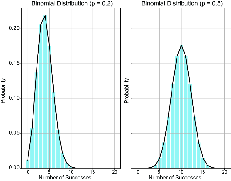
Compare distributions across twenty trials as p changes from 0.20 to 0.50; the plotted shape and location illustrate how the success probability affects outcomes. section 3.1.2





