Computational cost is the processing effort required by a function or algorithm. It is commonly understood through the number of operations needed as input size grows. Lower growth usually means better scaling, especially on large datasets. section 2.2
Big O notation gives a simple way to compare how operation counts grow:
- O(1) stays roughly constant, like shaking hands with one person regardless of the crowd. section 2.2
- O(n) grows with the input, like shaking hands with everyone in a room. section 2.2
- O(n²) compares every item with every other item, causing costs to rise rapidly. section 2.2
Cost is not the only practical concern. Memory use, hardware efficiency, parallel processing, energy consumption, and response latency can change which algorithm or model is preferable. A slower algorithm may still run faster when distributed across many processors, such as GPUs. section 2.2 section 11.11
Choosing an LLM architecture
Training a large language model with a huge vocabulary requires substantial processing power and energy. Larger architectures can capture more nuance, but training may require weeks or months on clusters of thousands of GPUs. The design therefore balances compute cost with memory capacity and latency: a capable model that takes too long to respond may not suit an interactive chatbot. section 11.11
Figure 2.3 Big O complexity
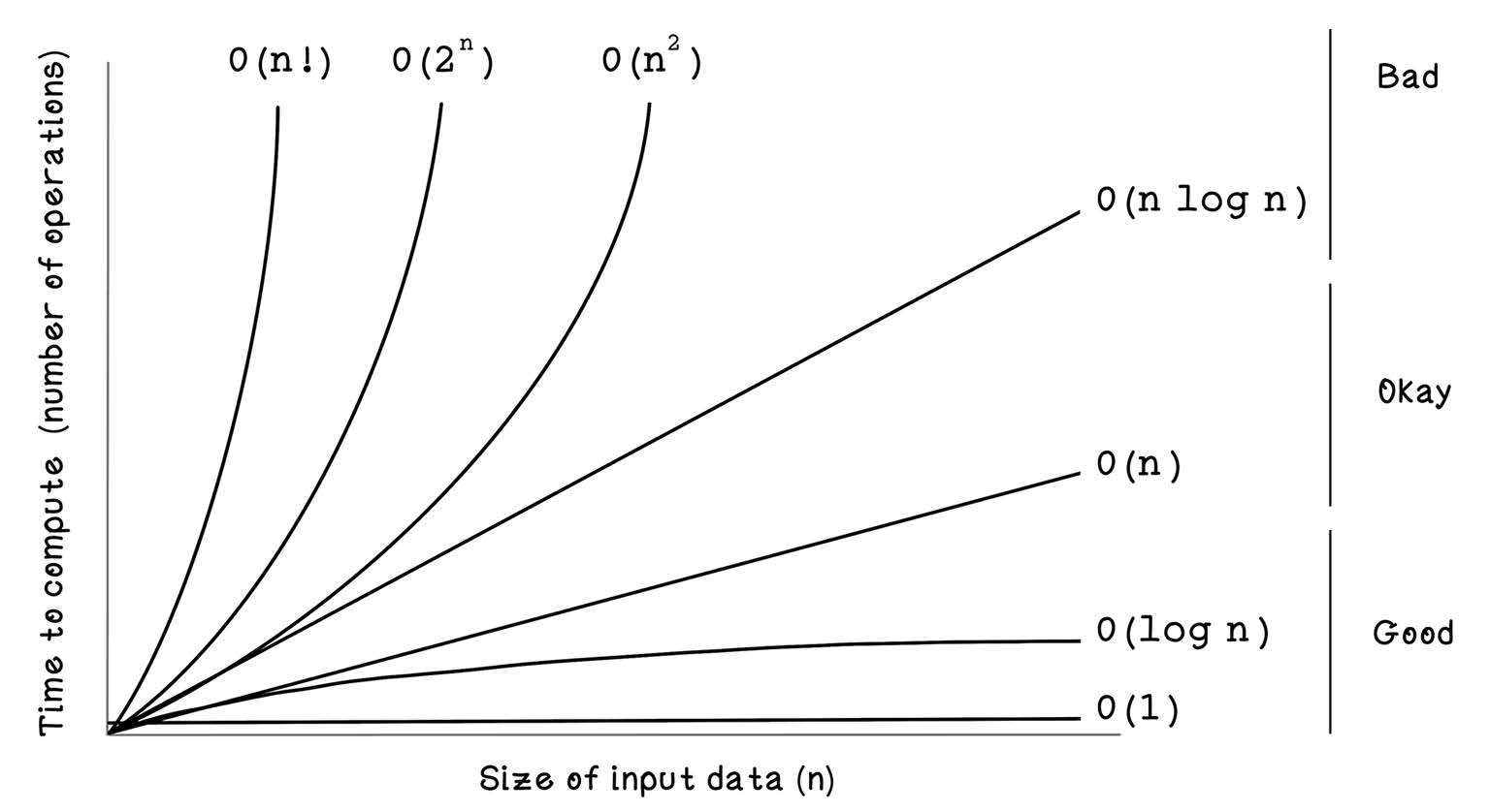
Compare how constant, linear, and quadratic operation counts grow as input size increases. section 2.2