Descriptive statistics summarize the observed features of a quantitative dataset. They help people understand a new data source, develop metrics, size an opportunity, or make a decision. A set of summaries may be a standalone dashboard or report; it may also provide context before an inferential statistical test. It describes the data at hand rather than, by itself, establishing what caused a difference. section 3.2.1 section 2.3.2
Choose measures to match the data and the question:
- For continuous values, use the mean, median, or mode to describe a typical value. The median is less affected by extreme values than the mean; a mode can highlight a concentration of values. section 4.1.1 section 4.1.2
- Describe spread as well as center. Standard deviation is useful for relatively symmetrical data; range and interquartile range can be more informative when a meaningful center is absent. section 4.1.1 section 4.1.2
- For categorical values, report counts or proportions. For activity over time, decide whether totals, per-user averages, or another aggregation answers the stakeholder’s question. section 3.2.1 section 2.1.3
Explore the data before settling on a number: check missing and duplicate records, then inspect the distribution’s shape. A single familiar average can conceal skew, outliers, or distinct patterns. Normality, a meaningful midpoint, and symmetry matter differently to different measures; check the relevant assumptions instead of treating every summary as interchangeable. Explain any aggregation that might surprise readers, and label charts and tables clearly. section 2.1.3 section 4.1.1 section 2.3.2
Figure 4.8 The mean (black dotted line) and median (gray dashed line) are approximately identical in the first and third distributions. The measures noticeably deviate in the second skewed distribution.
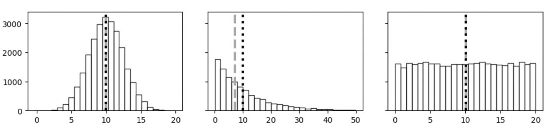
Compare the mean and median across three distributions: they are close in two, but diverge in the skewed one. The picture shows why inspecting shape should precede choosing an average. section 4.1.1
Choose the time unit and disclose its limits
For Help Center activity, calculate daily totals and their mean and median across the 90 days before and after a change, matching an established daily-volume metric. Weekly chart totals can make the trend easier to see when weekend activity drops, but readers should be told why the chart uses weeks. If customer satisfaction is available only as an overall average, show that average without implying that daily or row-level comparisons are available. section 2.3.2
Report more than one measure when one would mask an important property, and consider a distribution plot alongside the numbers. Check summaries before running statistical tests: a useful description of the observed data is not a substitute for evaluating a test’s assumptions or results. section 4.1.2 section 4.1.1





