A graph neural network (GNN) learns from relationships as well as features. It passes messages between nodes to capture dependencies in graph-structured data. Graph convolutional networks (GCNs) are one way to use this approach for node classification. section 11.7 section 11.4
Let G = (V, E) contain nodes V and edges E. Its adjacency matrix A records connections: Aᵢⱼ = 1 when an edge connects nodes i and j, and 0 otherwise. For an undirected graph, A is symmetric. If there are N nodes with F features each, the node-feature matrix X has shape N × F. Edges may also have features, represented by a matrix with one row per edge. section 11.4
Classifying documents in a citation graph
In the CORA citation network, nodes are documents and directed edges represent citations. A document’s features indicate which dictionary words it contains, giving X one row per document and one column per dictionary word. A GCN uses this feature-and-connection structure to classify nodes. That differs from assigning one label to an entire graph, as in molecule classification. section 11.4 section 11.4
The analogy with a convolutional neural network (CNN) is useful: an image can be viewed as a regularly structured graph whose pixels are nodes. Citation networks instead make their relationships explicit through edges. The graph and feature matrices establish what information is available to pass between nodes; they do not, by themselves, specify a GCN layer’s update rule. section 11.4 section 11.7
Listing 11.4 Graph convolutional neural network for classifying citation graphs
import numpy as np
import pandas as pd

import tensorflow as tf
from tensorflow import keras

import networkx as nx
from tensorflow.keras.utils import to_categorical
from sklearn.preprocessing import LabelEncoder
from sklearn.utils import shuffle
from sklearn.metrics import classification_report
from sklearn.model_selection import train_test_split

from spektral.layers import GCNConv

from tensorflow.keras.models import Model
from tensorflow.keras.layers import Input, Dropout, Dense
from tensorflow.keras import Sequential
from tensorflow.keras.optimizers import Adam
from tensorflow.keras.callbacks import TensorBoard, EarlyStopping
from tensorflow.keras.regularizers import l2

import os
from collections import Counter
from sklearn.manifold import TSNE
import matplotlib.pyplot as plt

tf.keras.utils.set_random_seed(42)

SAVE_PATH = "/content/drive/MyDrive/Colab Notebooks/data/"
DATA_PATH = "/content/drive/MyDrive/data/cora/"

column_names = ["paper_id"] + [f"term_{idx}" for idx in range(1433)] +
 ["subject"]
node_df = pd.read_csv(DATA_PATH + "cora.content", sep="\t", header=None,
 names=column_names)
print("Node df shape:", node_df.shape)

edge_df = pd.read_csv(DATA_PATH + "cora.cites", sep="\t", header=None,
 names=["target", "source"])
print("Edge df shape:", edge_df.shape)

nodes = node_df.iloc[:,0].tolist()
labels = node_df.iloc[:,-1].tolist()  #1
X = node_df.iloc[:,1:-1].values        #1

X = np.array(X,dtype=int)
N = X.shape[0] #the number of nodes
F = X.shape[1] #the size of node features

edge_list = [(x, y) for x, y in zip(edge_df['target'],
 edge_df['source'])]     #2

num_classes = len(set(labels))

print('Number of nodes:', N)
print('Number of features of each node:', F)
print('Labels:', set(labels))
print('Number of classes:', num_classes)

def sample_data(labels, limit=20, val_num=500, test_num=1000):
    label_counter = dict((l, 0) for l in labels)
    train_idx = []

    for i in range(len(labels)):
        label = labels[i]
        if label_counter[label]<limit:
            #add the example to the training data
            train_idx.append(i)
            label_counter[label]+=1

        #exit the loop once we found 20 examples for each class
        if all(count == limit for count in label_counter.values()):
            break

    #get the indices that do not go to traning data
    rest_idx = [x for x in range(len(labels)) if x not in train_idx]
    #get the first val_num
    val_idx = rest_idx[:val_num]
    test_idx = rest_idx[val_num:(val_num+test_num)]
    return train_idx, val_idx,test_idx


train_idx,val_idx,test_idx = sample_data(labels)

#set the mask
train_mask = np.zeros((N,),dtype=bool)
train_mask[train_idx] = True

val_mask = np.zeros((N,),dtype=bool)
val_mask[val_idx] = True

test_mask = np.zeros((N,),dtype=bool)
test_mask[test_idx] = True

print("Training data distribution:\n{}".format(Counter([labels[i] for i in
 train_idx])))
print("Validation data distribution:\n{}".format(Counter([labels[i] for i
 in val_idx])))

def encode_label(labels):
    label_encoder = LabelEncoder()
    labels = label_encoder.fit_transform(labels)
    labels = to_categorical(labels)
    return labels, label_encoder.classes_

labels_encoded, classes = encode_label(labels)

G = nx.Graph()
G.add_nodes_from(nodes)     #3
G.add_edges_from(edge_list)   #3

A = nx.adjacency_matrix(G)    #4
print('Graph info: ', nx.info(G))

# Parameters
channels = 16    #5
dropout = 0.5    #6
l2_reg = 5e-4     #7
learning_rate = 1e-2     #8
epochs = 200     #9
es_patience = 10     #10

# Preprocessing operations
A = GCNConv.preprocess(A).astype('f4')

# Model definition
X_in = Input(shape=(F, ))
fltr_in = Input((N, ), sparse=True)

dropout_1 = Dropout(dropout)(X_in)
graph_conv_1 = GCNConv(channels,
                       activation='relu',
                       kernel_regularizer=l2(l2_reg),
                       use_bias=False)([dropout_1, fltr_in])

dropout_2 = Dropout(dropout)(graph_conv_1)
graph_conv_2 = GCNConv(num_classes,
                       activation='softmax',
                       use_bias=False)([dropout_2, fltr_in])

# Build model
model = Model(inputs=[X_in, fltr_in], outputs=graph_conv_2)
model.compile(optimizer=Adam(learning_rate=learning_rate),
              loss='categorical_crossentropy',
              weighted_metrics=['accuracy'])
model.summary()

# Train model
validation_data = ([X, A], labels_encoded, val_mask)
hist = model.fit([X, A],
          labels_encoded,
          sample_weight=train_mask,
          epochs=epochs,
          batch_size=N,
          validation_data=validation_data,
          shuffle=False,
          callbacks=[
              EarlyStopping(patience=es_patience,  restore_best_weights=True)
          ])     #11

# Evaluate model
X_test = X
A_test = A
y_test = labels_encoded

y_pred = model.predict([X_test, A_test], batch_size=N)    #12
report = classification_report(np.argmax(y_test,axis=1),
 np.argmax(y_pred,axis=1), target_names=classes)
print('GCN Classification Report: \n {}'.format(report))

layer_outputs = [layer.output for layer in model.layers]
activation_model = Model(inputs=model.input, outputs=layer_outputs)
activations = activation_model.predict([X,A],batch_size=N)

#Get t-SNE Representation
#get the hidden layer representation after the first GCN layer
x_tsne = TSNE(n_components=2).fit_transform(activations[3])

def plot_tSNE(labels_encoded,x_tsne):
    color_map = np.argmax(labels_encoded, axis=1)
    plt.figure(figsize=(10,10))
    for cl in range(num_classes):
        indices = np.where(color_map==cl)
        indices = indices[0]
        plt.scatter(x_tsne[indices,0], x_tsne[indices, 1], label=cl)
    plt.legend()
    plt.show()

plot_tSNE(labels_encoded,x_tsne)

plt.figure()
plt.plot(hist.history['loss'], 'b', lw=2.0, label='train')
plt.plot(hist.history['val_loss'], '--r', lw=2.0, label='val')
plt.title('GNN model')
plt.xlabel('Epochs')
plt.ylabel('Cross-Entropy Loss')
plt.legend(loc='upper right')
plt.show()

plt.figure()
plt.plot(hist.history['accuracy'], 'b', lw=2.0, label='train')
plt.plot(hist.history['val_accuracy'], '--r', lw=2.0, label='val')
plt.title('GNN model')
plt.xlabel('Epochs')
plt.ylabel('Accuracy')
plt.legend(loc='upper left')
plt.show()
The citation-graph classification listing shows the practical stack, including TensorFlow/Keras and Spektral’s GCNConv layer. section 11.4
Figure 11.14 t-SNE hidden layer representation of the CORA dataset embedding after the first GCN layer
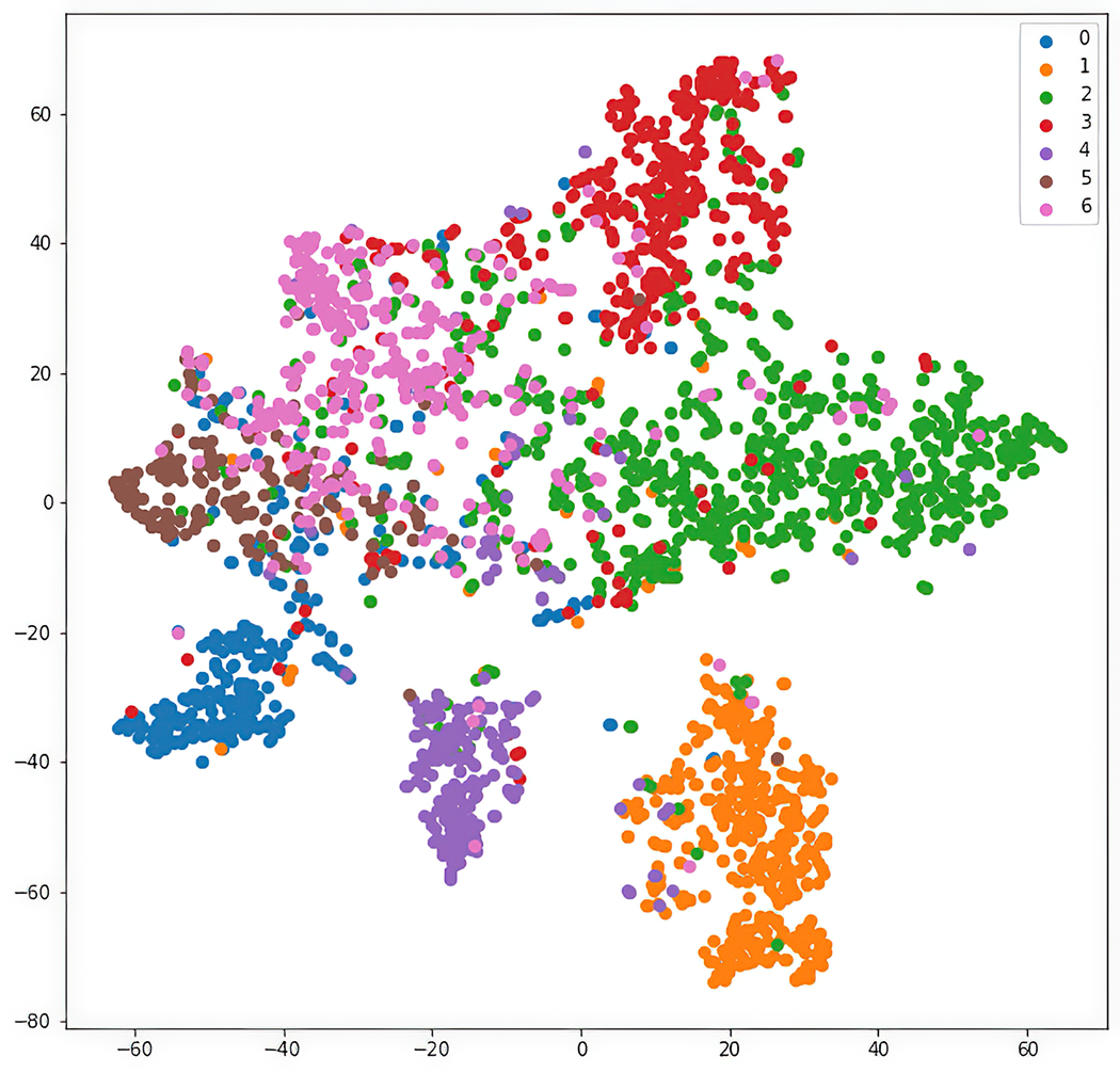
The t-SNE figure provides a way to inspect the CORA representation after the first GCN layer. section 11.4