Suppose a retailer wants customer groups it can inspect before deciding whom to target. Hierarchical clustering groups similar observations into a tree of nested clusters, called a dendrogram. It does not require a predefined number of final clusters: you choose where to cut the tree after examining it. That choice matters because the method does not identify an optimum number for you. section 2.4 section 2.6.4
The hierarchy can be built in either direction:
- Agglomerative clustering starts with each observation in its own cluster and repeatedly merges clusters from the bottom up. section 2.4.1
- Divisive clustering starts with one cluster and repeatedly splits it from the top down; this approach can take more time. section 2.4.1
Each merge or split makes a locally preferred choice without planning future steps. Distance matters, but so does the linkage method used to compare clusters. A dendrogram’s leaves represent observations; the height at which branches join helps you judge a distance cutoff. Different cutoffs can produce different numbers of clusters, so inspect the result rather than treating a visually appealing cut as definitive. section 2.4.1 section 2.4.4 section 2.4.5
Figure 2.20 Hierarchical clustering using average, ward, and complete linking methods (top to bottom, respectively)
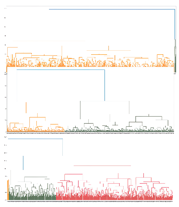
Compare the dendrograms produced by average, Ward, and complete linkage before choosing a method. section 2.4.5
Cut a dendrogram in Python
Start with a prepared, standardized feature array named X_standard. This example uses complete linkage and Euclidean distance, displays the last ten merges, then assigns clusters at a distance cutoff of 10: from scipy.cluster.hierarchy import dendrogram, linkage, fcluster import matplotlib.pyplot as plt Z = linkage(X_standard, 'complete', metric='euclidean') dendrogram(Z, truncate_mode='lastp', p=10) plt.show() clusters = fcluster(Z, 10, criterion='distance') print(len(set(clusters))) plt.scatter(X_standard[:, 0], X_standard[:, 1], c=clusters) plt.show() The cutoff of 10 yielded four clusters in the worked dataset; it is not a default for other data. Try other cutoffs and compare both the cluster count and the plot. section 2.4.5 section 2.4.5
For customer segmentation, first inspect transactions and customer attributes, address data-quality issues, and choose features such as visits, revenue, purchase categories, transaction channel, and age. Then compare candidate segmentations with business needs: examine cluster sizes and distinguishing attributes, and name groups only after interpreting their patterns. A cluster too small or too large to act on may need reconsideration. section 2.6.4
The tree is explainable and results are reproducible, but computation can be costly: the stated implementation cost is O(n³) time and at least O(n²) memory. Dendrogram cuts can also be subjective. Use the visualization to support a decision, then check that the resulting groups are useful in context. section 2.4.4 section 2.6.4