Hierarchical clustering

As explained in Statistics Slam Dunk

Hierarchical clustering is a clustering method that builds a nested hierarchy of groups based on similarity or distance.

Hierarchical clustering is an unsupervised method for finding structure in data without predicting a response variable. It starts with every observation in its own cluster, repeatedly merges similar clusters, and ends with one overall cluster. A dendrogram—an upside-down tree—shows the resulting nested hierarchy. section 3.9 section 20.1

Use it when a segmentation question calls for groups based on similarity and the number of groups is not known in advance. Unlike k-means clustering, it does not require an optimal cluster count beforehand, although it can become slow on large data sets. Common applications include customer segmentation using demographics and purchases, as well as biological and social-science analysis. section 3.9 section 20.1

A practical R workflow is:

• Select the variables that define similarity. For NBA draft selections, use pick number (Pk) and career win shares (WS), then calculate mean win shares for each first-round pick number. section 3.9
• Calculate Euclidean distances between the observations and store them in a distance matrix. section 3.9
• Run hclust() on that matrix, using complete linkage, then convert the result to a dendrogram and plot it. section 3.9
• Draw boxes for a chosen K to inspect a useful split in the hierarchy; K = 2 separates picks 1–5 from picks 6–30 in this analysis. section 20.1

Draft-pick career expectations

Mean career win shares for first-round selections in the 2000–2009 NBA drafts form a distance matrix across 30 pick numbers. The dendrogram’s two-cluster view places picks 1–5 together and picks 6–30 together, supporting different career expectations for top-five selections versus other first-round picks. section 3.9 section 20.1

Figure 3.7 A dendrogram that displays hierarchical clusters based on win shares and pick number

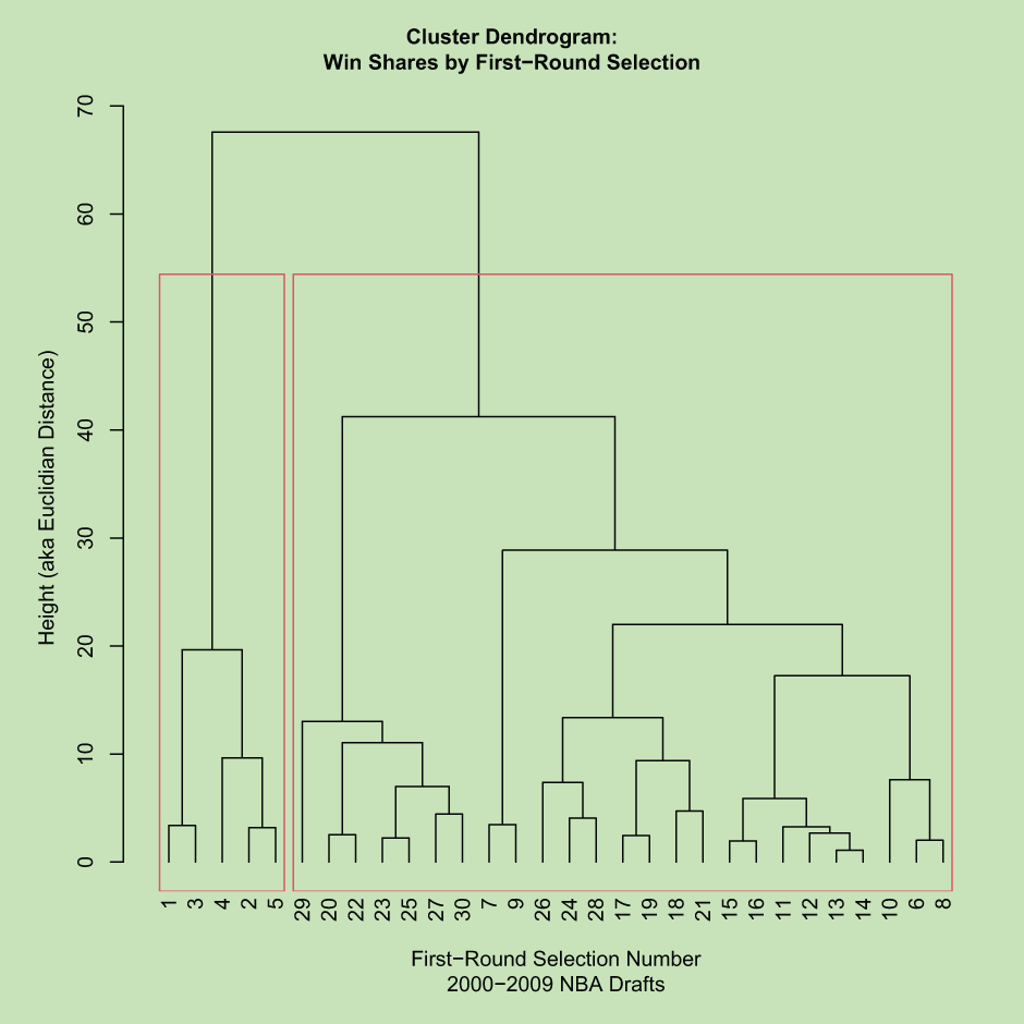
Inspect the dendrogram to see draft-pick clusters on the x-axis and their Euclidean-distance height on the y-axis. section 3.9

How Statistics Slam Dunk covers it

How deep it goes

Works through variable selection, mean aggregation, Euclidean distances, a distance matrix, complete-linkage hclust(), and dendrogram interpretation.

Examples

Uses 2000–2009 NBA first-round pick numbers and mean career win shares, highlighting a two-group split of picks 1–5 and 6–30.

What it assumes

Introduces clustering and unsupervised learning in plain language while requiring prepared numeric observations for similarity calculations.

What you can do after

Build it from scratch in base R by creating distances, running hclust(), plotting a dendrogram, and inspecting chosen cluster boxes.

How it connects

Connects unsupervised learning, cluster analysis, segmentation analysis, Euclidean distance, dendrograms, and k-means clustering.

liveBookmanning.com

Read Statistics Slam Dunk on liveBook Get the book at manning.com

Also explained in

• 

  liveBookmanning.com
  Data Without LabelsHierarchical clustering is a clustering method that constructs a nested hierarchy of groups by successively merging or splitting clusters.
• 

  liveBookmanning.com
  Build a Robo-Advisor with Python (From Scratch)Hierarchical clustering is a clustering technique that organizes objects into progressively combined or subdivided groups according to a distance measure.
• 

  liveBookmanning.com
  Advanced Algorithms and Data StructuresHierarchical clustering is a clustering technique that forms nested groups by successively merging or dividing clusters.
• 

  liveBookmanning.com
  Domain-Specific Small Language ModelsA clustering approach that builds communities through repeated refinement and aggregation of grouped items.

Compare how 5 books explain hierarchical clustering →

Related concepts

• K-means clusteringcontrasts with · K-means clustering partitions data into a specified number of groups by assigning observations to representative centers and iteratively updating those centers to reduce within-group distances.
• OPTICSincludes · OPTICS is a density-based clustering algorithm that orders points and computes reachability distances to reveal cluster structure across varying density thresholds.
• unsupervised learningkind of · Unsupervised learning is a machine-learning approach that discovers patterns, structure, or representations in data without labeled target outputs.
• clusteringkind of · Clustering is the technique of grouping data items according to similarity or shared characteristics.
• agglomerative clusteringincludes · Agglomerative clustering is a bottom-up hierarchical clustering method that starts with individual items as separate clusters and repeatedly merges clusters according to a linkage criterion.

This explainer was generated by Manning's knowledge graph from the text of Statistics Slam Dunk. The section links point to the parts of the book it draws on.