Interpolation constructs a function whose graph passes exactly through a specified set of data points. Unlike ordinary approximation, which may deliberately miss points to show an overall trend, interpolation has zero error at the interpolation points. That exactness is especially useful in geometry: curves and surfaces must meet cleanly, without gaps where separate pieces join. section 6.0 section 6.3
Figure 6.18 When a polynomial approximates the data set with 0 error, every data point belongs to its graph.
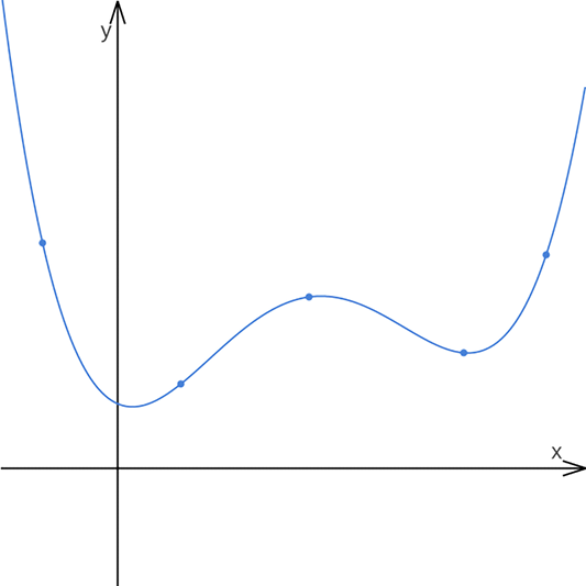
An interpolating polynomial contains every input point on its graph; this is the visual meaning of zero fitting error. section 6.3
Polynomial interpolation commonly represents N data points with a polynomial of degree N−1, although higher degrees are possible. A least-squares method can produce an interpolating polynomial, but solving through a Vandermonde matrix is presented as the more practical computation. Lagrange interpolation offers another form, mainly for understanding basis polynomials. section 6.3.6 section 6.7
Choose the interpolating form to match the job rather than treating exact fitting as a universal modeling solution:
- Use polynomial interpolation to construct curves and surfaces that must pass through designated points exactly. section 6.0
- Use inverse-distance interpolation for scattered values in two or three dimensions; weights are inverse powers of Euclidean distance, and increasing the power makes plateaus more pronounced. section 8.3.2
- Use linear interpolation in marching squares or cubes when estimating an implicit surface crossing on a cell edge; it is quick enough for large triangle counts. section 11.3.1
- Prefer approximation when a global trend matters more than hitting every measured value, because an exact interpolant can suggest the wrong process model. section 6.4
Interpolating scattered spatial values
Given points (xs[i], ys[i]) with values vs[i], define F(x, y) as a weighted average of the values. For each sample, compute its distance to (x, y), return its stored value when the distance is zero, and otherwise weight that value by the reciprocal of distance raised to a chosen power. The same pattern extends directly to three variables and can use any number of points. section 8.3.2
Smooth deformation from control vectors
A deformation field can be made by interpolating random displacement vectors from control points around a model. Evaluate separate three-variable interpolants for x, y, and z at every model point, then add the resulting vector. Continuous, smooth interpolation produces a continuous, smooth deformation, allowing varied mushroom shapes without visible breaks. section 8.3.4
Interpolation can also turn a finite image grid into a continuous function of two variables. After subtracting a light/dark threshold, that function can guide iterative contour fitting. It is not a true signed distance function, so its values are only suggested translation distances; an approximation threshold determines when fitted vertices are close enough to the target contour. section 12.4.3
Exactness does not guarantee a faithful real-world model. Interpolation is valuable for constructing clean geometric representations, while deciding whether a fitted function describes an underlying process remains a modeling question. Polynomial methods are a useful foundation for polynomial splines, while multivariable problems can call for nonpolynomial spatial approaches. section 6.4 section 8.3