Interpolation estimates a business metric at unmeasured settings between nearby measured values. It relies on a continuity assumption: small changes in a continuous parameter should produce small changes in the metric. This makes it useful when evaluating every possible threshold, weight, or other parameter value would be too costly. In response surface methodology, interpolation turns aggregate measurements into a surrogate function that approximates the underlying response surface, then supports a search for better parameter settings. section 4.1.1 section 4.3
With two measurements, use a line segment between them. If threshold=1 produces profit 5 and threshold=2 produces profit 6, the midpoint threshold=1.5 receives the estimate (5+6)/2=5.5. This estimate is most defensible for unmeasured values close to the observed endpoints. Two points cannot reveal an interior optimum: a straight-line interpolation always reaches its maximum at one measured endpoint. section 4.1.1 section 4.2.1
Fit a one-parameter surrogate
For three aggregate profit measurements, fit a quadratic model, y-hat=β0+β1x+β2x², by linear regression. The fitted parabola interpolates between measured thresholds and can have a maximum at an unmeasured threshold. A NumPy implementation builds a design matrix containing constant, linear, and squared threshold terms, solves for β, then evaluates the model over a closely spaced range between the smallest and largest measured thresholds. With exactly three measurements and three model parameters, the quadratic fits those measurements exactly; with additional measurements, approximation error is expected. section 4.1.3
Design measurements around the interpolation you need:
- Measure at least three values of a parameter when seeking a maximum between lower and upper bounds; the third measurement buys the ability to fit a curved surrogate rather than only a line. section 4.2.1
- For two parameters, measure values along both dimensions and use a quadratic model with linear, squared, and cross terms; the cross term models behavior along design diagonals. section 4.2.2
- Use a central composite design with corner points when interpolation must work across the full two-dimensional region, not only near its center and edges. section 4.2.1
- Treat unusual measurements as a warning that the local-near-optimum modeling assumption may be violated; redesign and remeasure before trusting optimization. section 4.2.2
- Validate the estimated optimum with a final measurement. If its result falls outside the measurement's 95% confidence bounds, return to design and iterate. section 4.2.2
Figure 4.18 A two-dimensional surrogate function, an interpolation of markout_profit_2D over settings of threshold and order_size. The filled dots mark the parameter settings where markout profit was measured in the experiment. In this figure, there are many more estimates of markout profit (around 20,000 interpolation estimates) than measurements (only nine).
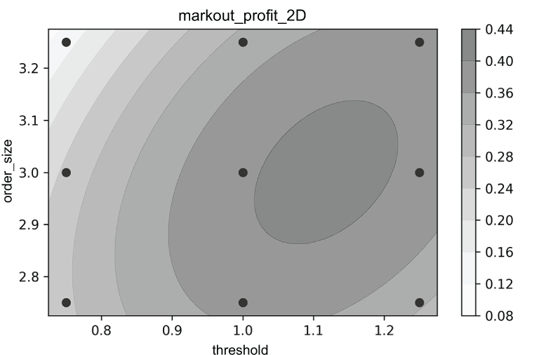
A two-dimensional surrogate expands nine measured threshold/order-size settings into roughly 20,000 estimated profit values, making the response surface and its search space visible. section 4.2.2
Interpolation reduces experimentation cost because optimization can search the surrogate rather than directly measure every setting. Its result remains an estimate, not a replacement for measurement: select ranges that cover the likely optimum, fit locally where the model assumptions are plausible, inspect measurements for outliers, and validate the final recommendation. Iteration is part of the method when the current design does not adequately locate or confirm an optimum. section 4.2.2 section 4.3