Poisson distribution

As explained in Causal AI

The Poisson distribution gives the probabilities of the number of events occurring in a fixed interval under a constant-rate event process.

The Poisson distribution models the number of events occurring within a fixed time period when the event's waiting time follows an exponential distribution. Its outcomes are discrete, begin at zero, and have no upper bound; probabilities taper as counts increase. section 2.3.1 section 2.1.8

Choose it by reasoning from the stochastic process that generated the population, rather than treating the distribution as an isolated formula. This connects canonical distributions to generative and causal modeling workflows. section 2.3.1

Use the distribution to:

• Visualize count probabilities with a bar plot, distinguishing the result from a histogram. section 2.1.8
• Compare a discrete Poisson distribution with a continuous normal approximation when their shapes overlap. section 2.1.8
• Generate samples inside probabilistic programs, including a Poisson latent variable in Pyro. section 2.3.1

Figure 2.12 A continuous normal distribution (solid line) approximates a discrete Poisson distribution (gray bars). Again, the outcomes are on the horizontal axis, and the probability values are on the vertical axis.

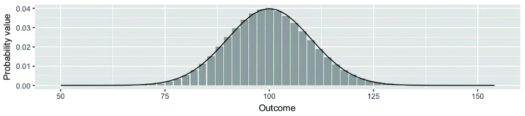
Compare the Poisson bars with a continuous normal curve to inspect how a count distribution can be approximated visually. section 2.1.8

How Causal AI covers it

How deep it goes

Explains outcome support, tapering probabilities, process selection, visualization, and sampling, but does not develop the probability mass formula.

Examples

Uses bar plots, a Poisson-normal overlay, and Pyro code that samples a Poisson latent variable.

What it assumes

Assumes familiarity with probability distributions and stochastic processes while connecting waiting times to event counts.

What you can do after

Apply it via Pyro to represent count generation inside a probabilistic model.

How it connects

Connects exponential distribution, stochastic processes, probability distributions, generative modeling, causal modeling, and IID sampling.

liveBookmanning.com

Read Causal AI on liveBook Get the book at manning.com

Also explained in

• 

  liveBookmanning.com
  Statistics Every Programmer NeedsThe Poisson distribution gives the probabilities of observing specified counts of events in a fixed interval when events occur independently at a constant average rate.
• 

  liveBookmanning.com
  Ensemble Methods for Machine LearningA Poisson distribution is a discrete probability distribution for the number of events occurring in a fixed interval under a constant-rate event process.
• 

  liveBookmanning.com
  Machine Learning System DesignA probability distribution for the count of events occurring independently at a constant average rate in a fixed interval or exposure.
• 

  liveBookmanning.com
  Machine Learning for Tabular Data: XGBoost, Deep Learning, and AIThe Poisson distribution models the number of events occurring in a fixed interval when events occur independently at a constant average rate.
• 

  liveBookmanning.com
  Natural Language Processing in Action, Second EditionA Poisson distribution is a probability distribution for counting events in a fixed interval given a specified average rate.
• 

  liveBookmanning.com
  Grokking StatisticsThe Poisson distribution is a discrete probability distribution for the number of events occurring in a fixed interval under a constant-rate independent-event assumption.

Compare how 7 books explain Poisson distribution →

Related concepts

• probability distributionkind of · A probability distribution is a mathematical specification assigning probabilities to the possible values or outcomes of a random variable, with total probability one.
• Poisson regressionused by · Poisson regression is a generalized linear model for count or rate outcomes using a Poisson response distribution and typically a log link.
• rate parameterhas part · A rate parameter is a parameter that controls the frequency or rate of events or outcomes in a probability distribution.
• exponential distributioncontrasts with · The exponential distribution is a continuous probability distribution over nonnegative values with an exponentially decreasing density, commonly modeling waiting times between events in a constant-rate Poisson process.
• discrete distributionkind of · A discrete probability distribution assigns probability mass to outcomes in a finite or countably infinite set of distinct values.
• binomial distributionalternative to · A binomial distribution is the probability distribution of the number of successes in a fixed number of independent trials, each with the same probability of success.

This explainer was generated by Manning's knowledge graph from the text of Causal AI. The section links point to the parts of the book it draws on.