A dataset with hundreds of variables can be difficult to visualize and slow to analyze, especially when variables are correlated. Principal component analysis (PCA) reduces its dimensions by projecting the data onto new variables called principal components. Each component is a linear combination of the original variables. The first captures the greatest variance; later components capture further variance while remaining orthogonal to earlier ones. section 3.5 section 3.7
Think of the components as directions through the data. A useful first direction captures substantial variation with relatively small projection errors. A second, perpendicular direction captures variation the first did not. Keeping only the leading directions gives fewer columns while retaining much of the dataset’s variation—not every detail of the original variables. section 3.5 section 3.7
Figure 3.8 The first figure on the left is the first principal component. The second principal component can be at different angles with respect to the first principal component (middle). We should find the second principle that allows us to capture the maximum variance. To capture the maximum variance, the second principal component should be orthogonal to the first one, and thus the combined variance captured is maximized (right).
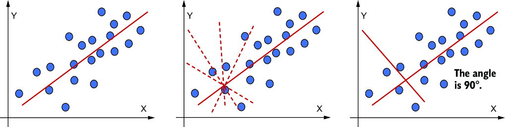
The diagram contrasts possible second components and shows why the chosen direction is perpendicular to the first. section 3.5
A practical Python workflow is:
- Inspect the rows, columns, and variable ranges; separate any target column from the features. Clean unsuitable values, convert categorical features to numeric form, and standardize the features. section 3.5.2 section 3.7
- Fit `sklearn.decomposition.PCA` to the standardized features. For a closer look at the mathematics, form their covariance matrix and calculate its eigenvalues and eigenvectors. section 3.5.2
- Plot `explained_variance_ratio_` by component and cumulatively. Use those views to choose how many components retain enough variance for the task, then transform the features and inspect the result. section 3.5.2
Iris flowers in two dimensions
The Iris example starts with 150 flowers and four measured properties used as features; species is kept separately as the target. After standardization, a two-component PCA produces a two-column representation without changing the number of flowers. A scatter plot colors the projected points by species so the result can be inspected visually. Explained-variance and cumulative-variance plots help assess what was retained. section 3.5.2
For a telecommunications customer dataset, demographic, subscription, usage, and payment attributes can accumulate into a large feature set. First check for missing, duplicate, sparse, or uninformative data; then consider reducing attributes before clustering or supervised modeling. PCA can simplify visualization and computation, but its combined components may be hard to explain in business terms, and discarded components can contain useful information. It is a linear method: nonlinear alternatives such as UMAP may better capture more complex patterns. section 3.8 section 3.7 section 6.5.3









