Principal component analysis (PCA) transforms features into components that capture decreasing amounts of variance. When features are correlated, a few components can represent much of the data. This makes PCA useful for reducing dimensions and visualizing data, but the transformed space can also reveal outliers hidden by the original feature values. section 6.9
Two ways to depart from a pattern
Imagine observations clustered along a diagonal in a two-feature plot. One unusual point lies far along that diagonal; another has ordinary values in both features but falls away from it. PCA aligns the first component with the dominant pattern and the second with the remaining variation. The first point is extreme on the major component, while the second stands out on the minor one. section 6.9
Figure 6.13 The left pane shows the original data, which contains two outliers, one (point A) that keeps with the general pattern of the data but is extreme and one that has typical values in both dimensions but does not keep with the general pattern (point B). The right pane shows the two components after PCA transformation, with the first component (which captures most of the variance) on the x-axis and the second component (which captures the remaining variance) on the y-axis. The outliers stand out as extreme values in the two components.
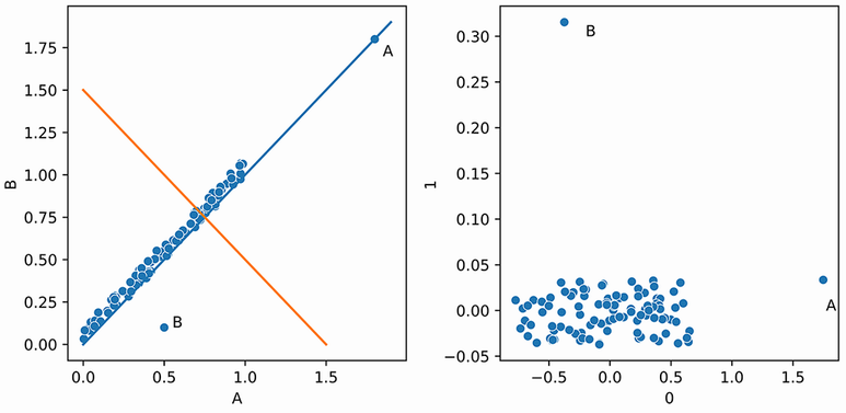
Compare the original coordinates with the transformed coordinates to see how different kinds of outlier become extreme on different components. section 6.9
One approach is to apply univariate outlier tests to selected components. Early components describe major patterns; later components can expose deviations from those patterns. Which components matter depends on the outliers sought. Equal weighting is a starting point, but component selection and weights can be adjusted as flagged cases are reviewed. Looking only at the components with the most variance may miss useful signals in the last ones. section 6.9.1 section 10.1.1
A PCA-based detector can instead score reconstruction error: it measures how far a point lies from the space represented by the first k components. Points poorly represented by that space receive higher outlier scores. PyOD’s PCA detector uses this approach for linear relationships; its KPCA alternative is recommended when those relationships are not linear. Obvious outliers should be removed before fitting, because the model needs to learn the usual pattern. section 6.9.3
Listing 6.10 Using ECOD to clean data before using PCA for outlier detection
import pandas as pd
from pyod.models.pca import PCA
from pyod.models.ecod import ECOD
from sklearn.datasets import fetch_openml

data = fetch_openml(“speech”, version=1, parser='auto')       #1
df = pd.DataFrame(data.data, columns=data.feature_names)
scores_df = df.copy()

clf = ECOD(contamination=0.01)                                #2
clf.fit(df)
scores_df['ECOD Scores'] = clf.predict(df)

clean_df = df[scores_df['ECOD Scores'] == 0]                  #3

clf = PCA(contamination=0.02)                                 #4
clf.fit(clean_df)
pred = clf.predict(df)                                        #5
The Python example removes the top 1% flagged by ECOD, fits a PyOD PCA detector to the cleaned rows, then predicts on the full dataset. section 6.9.3
As preprocessing, PCA can reduce the number of features passed to another detector, potentially speeding detection and making two- or three-dimensional plots possible. Test the choice rather than assuming a gain: compare original features, all components, and selected early or late components on both runtime and known outlier rankings. Components may make an outlier easy to see without making its original-feature explanation clear. With very few rows and many features, even PCA-based results risk being spurious; restrict analysis to a small number of relevant components when strong linear patterns justify it. section 10.1.1 section 10.3









