Principal component analysis (PCA) finds the directions in multivariate data along which points vary most. It replaces the original coordinate system with orthogonal principal axes, ordered from greatest to least spread. The coordinates on those axes are principal components, and their variances are principal values. PCA is useful when high-dimensional points lie near a lower-dimensional line, plane, or hyperplane: retaining the large-variance directions preserves the main pattern while discarding small variations. section 4.1 section 4.4.1
Begin with centered data. In one dimension, spread around the mean is variance. In several dimensions, spread depends on direction, so the covariance matrix captures both per-axis variation and joint variation. For a unit direction l̂, the variance of the projected data is l̂ᵀCl̂, a quadratic form. Maximizing this quantity selects the covariance-matrix eigenvector with the largest eigenvalue; that eigenvector is the first principal axis, and the eigenvalue is its principal value. Subsequent eigenvectors give mutually orthogonal directions with the next-largest variances. section 4.4 section 4.7
A PCA workflow is:
- Arrange instances as rows of a data matrix and subtract the mean of each feature. section 4.5.3 section 14.4.1
- Compute covariance-matrix eigenvalues and eigenvectors, or compute an SVD of the centered data matrix. section 4.4.3 section 4.5.7
- Sort directions by decreasing principal value and retain the leading axes appropriate for the desired representation. section 4.4.1 section 4.4.2
- Project data onto the retained axes; optionally reconstruct an approximate original-space point from that reduced representation. section 4.4.5 section 14.4.1
Reducing a nearly linear 2D cloud
For points concentrated near y = 2x, one principal value is far larger than the other. The leading principal vector follows the cloud’s main line, while the orthogonal direction captures relatively small deviations. Projecting each 2D point onto the leading axis creates a 1D representation with little information loss. By contrast, uncorrelated 2D data has two large principal values, so reducing it to one dimension is not effective. section 4.4.3 section 4.4.2
Figure 4.3 Dimensionality reduction via PCA. Original data points are shown with filled little circles, and hollow circles represent lower-dimensional representations.
|
(a) Dimensionality reduction from 2D to 1D |
|
(b) Dimensionality reduction from 3D to 2D |
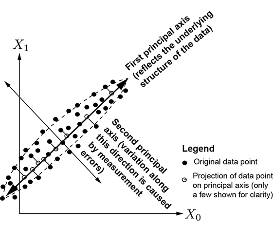
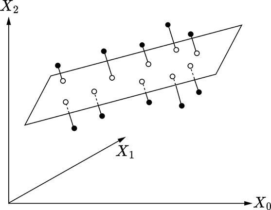
Compare 2D-to-1D and 3D-to-2D projections to see how small-variance perpendicular components are removed. section 4.4.2
PCA supports dimensionality reduction and compression by storing projections on only the first few principal axes. Small-principal-value components are often treated as noise or minor perturbations, though this is an interpretation rather than a guarantee. PCA is linear: when points follow a curved pattern, projecting them onto a straight principal axis can produce substantial positional error and lose important structure. section 4.4.5 section 4.4.4
SVD supplies another route to PCA. For mean-subtracted data X with instances as rows, XᵀX is the covariance matrix as presented here. The right singular vectors of X provide principal vectors, while singular values provide principal values, making SVD a practical computation method. In PyTorch, this can be expressed with torch.linalg.svd after centering the data, then selecting leading columns of V for projection. section 4.5.3 section 14.4.1









