A probability density describes the relative likelihood of outcomes for a continuous random variable. Unlike a discrete probability mass, it does not assign probability directly by summing individual outcomes; integrating the density over an interval gives that interval’s probability. Across all possible values, the integral equals one. section 2.1.1 section 2.1.7
Use the distinction between mass and density to interpret probabilistic models:
- For discrete variables, P(X = x) gives the probability of a specific outcome, and probabilities sum to one. section 2.1.1 section 2.1.7
- For continuous variables, a density describes relative likelihood across a range; integration, rather than pointwise summation, produces probability. section 2.1.1 section 2.1.7
- Canonical continuous distribution classes, such as the normal and gamma families, become specific distributions after parameters are assigned. section 2.1.7
A parameterized distribution in Pyro
A normal distribution can be instantiated with loc=0.0 and scale=1.0, while a gamma distribution can use concentration=1.0 and rate=2.0. These parameter values turn distribution classes into concrete probabilistic objects. section 2.1.7
Figure 2.10 A popular common set of canonical probability distributions. The edges capture mathematical relationships between the distributions (that we won’t get into here). Light-colored distributions are discrete and dark-colored distributions are continuous. An arrow represents the existence of a transformation that converts one distribution to another.
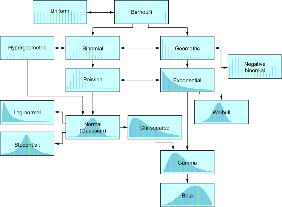
Use the distribution map to distinguish continuous families from discrete ones and to see their stated transformation relationships. section 2.1.7





