Probability density

As explained in Statistics Every Programmer Needs

A probability density function describes the relative likelihood of values of a continuous random variable, with probabilities obtained over intervals rather than at individual points.

A probability density function (PDF) describes the relative likelihood of values taken by a continuous random variable. Its formula depends on the modeled distribution, and its curve shows density across possible values. section 2.3.2 section 3.1.1

A density value is not itself the probability of observing one exact continuous value. Probabilities come from the area under the curve across an interval, such as the range between standardized values 1.0 and 1.5. section 2.3.2 section 3.1.1

For a normal distribution, the PDF is determined by the mean μ and standard deviation σ. The curve is symmetric and bell-shaped, peaks at the mean, and becomes flatter and more dispersed as σ increases. section 3.1.1

Use the normal PDF computationally in two equivalent ways:

• Evaluate the formula directly with μ, σ, and a value z; for μ = 0, σ = 1, and z = 1, the density is approximately 0.24197. section 3.1.1
• Call scipy.stats.norm.pdf(z, loc=μ, scale=σ) for the same density, then use norm.cdf to obtain cumulative probability or subtract CDF values for an interval. section 3.1.1
• Generate normal samples with NumPy and compare observations within one, two, and three standard deviations of the mean. section 3.1.1

Standard normal density and interval area

For the standard normal distribution, μ = 0 and σ = 1. Evaluating the PDF at z = 1 gives 0.2419707245. The cumulative probability below z = 1 is about 84.13%; below z = 1.5 it is about 93.32%, so the probability between them is about 9.18%. section 3.1.1

Figure 2.2 The normal distribution illustrates where the interval, or range of possible values—which runs along the x axis—equals [2, 6]. The probability density, which runs along the y axis, peaks at the mean and typically tops out at approximately 0.399. The probability density for any value can therefore be estimated merely by observation. When the value equals 3.2, the probability density appears to be equal to approximately 0.30.

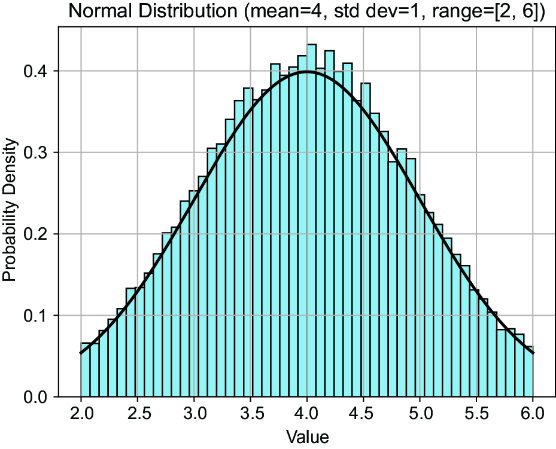
Inspect the normal curve for the interval [2, 6], where density peaks near the mean and is approximately 0.30 at 3.2. section 2.3.2

How Statistics Every Programmer Needs covers it

How deep it goes

Defines PDFs, explains normal-distribution parameters, and demonstrates direct, SciPy, NumPy, and CDF calculations.

Examples

Uses normal curves, standard-normal calculations, NumPy samples, and probabilities between z = 1.0 and z = 1.5.

What it assumes

Assumes basic continuous-variable and mean concepts while defining density, standard deviation, and standardization in context.

What you can do after

Apply via SciPy's norm.pdf and norm.cdf, or reproduce normal-density calculations with Python and NumPy.

How it connects

Connects continuous random variables with normal distributions, standard deviation, standardization, z-scores, and cumulative probability.

liveBookmanning.com

Read Statistics Every Programmer Needs on liveBook Get the book at manning.com

Also explained in

• 

  liveBookmanning.com
  Math and Architectures of Deep LearningA function describing probability density for continuous-valued distributions.
• 

  liveBookmanning.com
  Fabulous Adventures in Data Structures and AlgorithmsA probability density function is a nonnegative function whose integral over a range determines the probability of a continuous random variable falling in that range.
• 

  liveBookmanning.com
  Grokking StatisticsA probability density function is a function whose values describe the relative likelihood of values of a continuous random variable.
• 

  liveBookmanning.com
  Causal AIA probability density is a nonnegative function describing the distribution of a continuous random variable, whose integral over all possible values is one.
• 

  liveBookmanning.com
  Statistics Slam DunkA probability density function describes the relative likelihood density of a continuous random variable across its range.

Compare how 6 books explain probability density →

Related concepts

• probability theorycontrasts with · Probability theory is the branch of mathematics that formalizes uncertainty and analyzes random events and outcomes using probability measures.
• cumulative distribution functionproduces · A cumulative distribution function gives the probability that a random variable is less than or equal to each specified value.
• density plotused by · A density plot is a visualization that estimates and displays the shape of a continuous variable’s probability distribution as a smooth curve.
• violin plotused by · A violin plot is a statistical visualization that represents the distribution of numeric data with a mirrored, smoothed density shape, often accompanied by summary statistics.
• probability distributionconfigured by · A probability distribution is a mathematical specification assigning probabilities to the possible values or outcomes of a random variable, with total probability one.

This explainer was generated by Manning's knowledge graph from the text of Statistics Every Programmer Needs. The section links point to the parts of the book it draws on.