A probability density describes how strongly a continuous distribution supports values along its x-axis. Its height is not itself a probability: probabilities come from the area under the curve across a range of values. The total area under a continuous distribution is 1.0. section 3.8 section 4.5
This differs from a discrete distribution, where bar heights can represent probabilities and be summed. For a continuous value, asking for the probability of one exact value is not useful; ask for an interval instead, such as a success rate between 0.4 and 0.7 or a dog weight between 61 and 63 pounds. section 3.8 section 4.5
Use a density curve to calculate an interval probability:
- Plot density values with a PDF, such as scipy's beta.pdf() or norm.pdf(). section 3.8 section 4.4
- Use a CDF to get the area from the left edge of the distribution up to a value. section 3.8 section 4.5
- Subtract the CDF at the lower bound from the CDF at the upper bound to get the area, and therefore probability, between them. section 3.8 section 4.5
A probability between two dog weights
With a normal distribution whose mean is 64 pounds and standard deviation is 3 pounds, the density at 61.63 pounds is only a curve height. The probability that a golden retriever weighs from 61 to 63 pounds is the shaded area in that interval: norm.cdf(63, 64, 3) - norm.cdf(61, 64, 3) = 0.2108, or 21.08%. section 4.5
Figure 4.6 Looking up the probability/area for a golden retriever between 61 and 63 pounds
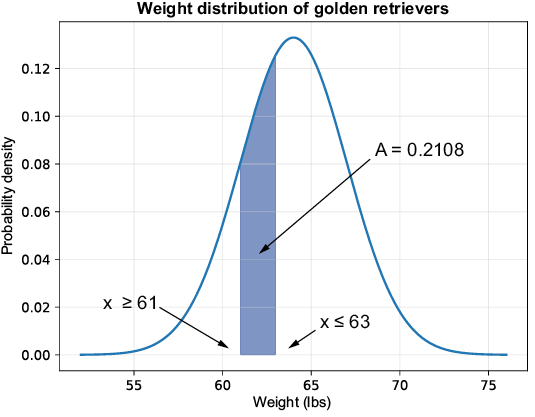
The shaded band shows the key distinction: the probability is the area between 61 and 63 pounds, not the density value at either point. section 4.5





