Propensity score

As explained in Causal Inference for Data Science

A propensity score is the conditional probability that a unit receives a treatment given its observed covariates.

A propensity score is the conditional probability that a unit receives treatment given its observed confounders: S(c) = P(T = 1 | C = c). It turns a potentially long description—age, sex, location, and other confounders—into one value describing how likely that type of unit was to be treated. section 5.2.2 section 5.2.1

The practical question is not simply whether treated and untreated groups have different outcomes, but whether they contain comparable cases. If doctors avoid a newer treatment for older patients, age affects both treatment assignment and recovery, so a raw difference in average outcomes cannot estimate the average treatment effect (ATE). section 5.1 section 5.0

From patient types to comparable scores

Suppose four of five young patients receive treatment, giving PS(young) = 4/5, while one of four older patients receives it, giving PS(old) = 1/4. Rather than requiring exact matches on every covariate, compare units with similar scores. Categories such as children and older patients can be combined when they share a propensity score, because their treated/control composition is comparable for estimating an ATE. section 5.1.4 section 5.2.2

Propensity scores are especially useful with many confounders, where matching directly on every combination of covariates becomes difficult. Estimate each unit's treatment probability from a dataset containing treatment status and confounder columns; logistic regression is common, while random forests, boosting, and other classifiers can also be used. section 5.3.2 section 5.2.1

A practical propensity-score workflow is:

• Explore the population and identify subgroups assigned to only treatment or only control; discard them when appropriate. section 5.2
• Estimate treatment probabilities from observed confounders, using predicted probabilities rather than predicted treatment labels. section 5.3.2
• Inspect score distributions by treatment group to assess positivity and find the common support where matches exist. section 5.2 section 5.3.3
• Calculate ATEs only when groups are comparable, or restrict the analysis to the overlapping subset. section 5.2 section 5.3.3

Figure 5.10 Full overlap between distributions' supports. This is the ideal scenario to calculate ATEs.

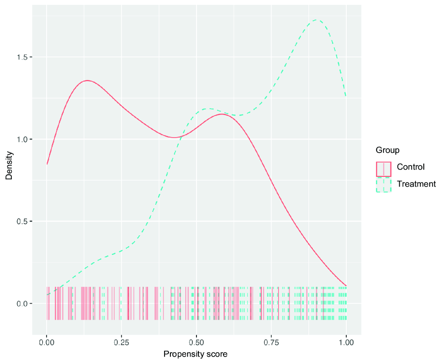
Compare the treated and control score distributions. Full overlap is the ideal setting for estimating an ATE; no overlap means there are no comparable matches. section 5.3.3

Positivity requires 0 < P(T = 1 | c) < 1 for every relevant covariate pattern. A score of 0 or 1 means that type of patient appears in only one treatment group, so its counterfactual outcome cannot be compared. Partial overlap can still support an effect estimate for the common-support population, and overlap limited to treated units can support an ATT. section 5.1.2 section 5.3.3

A propensity score is an adjustment-formula tool, not evidence that all confounding has disappeared. It is calculated from a chosen confounder set; for causal adjustment, that set must satisfy the back-door criterion. Conditional on a score, the treatment is independent of the included covariates, so the score summarizes their treatment-assignment information and blocks the corresponding back-door paths. section 7.4.2 section 5.2.2

Cross-fitted clinical analysis

For the Right Heart Catheterization dataset, estimate each patient's probability of receiving RHC from selected confounders. To reduce overfitting, split the data in two: fit the propensity model on one half and predict scores on the other, then reverse the roles. Plot score densities by treatment group before using cross-fitted estimates in an ATE analysis. section 5.4 section 5.4.1

How Causal Inference for Data Science covers it

How deep it goes

Defines the score, explains grouping and overlap, and practices machine-learning estimation with cross-fitting; defers specialized theory.

Examples

Uses age-based patient groups, a surgical-treatment scenario, and Right Heart Catheterization survival data.

What it assumes

Assumes familiarity with confounders, treatment and outcome variables, ATEs, and the adjustment formula while introducing score notation from zero.

What you can do after

Apply it via logistic regression or other classifiers to inspect overlap and estimate effects for comparable populations.

How it connects

Connects propensity scores to confounders, positivity, matching, the adjustment formula, ATE, ATT, and the back-door criterion.

liveBookmanning.com

Read Causal Inference for Data Science on liveBook Get the book at manning.com

Also explained in

• 

  liveBookmanning.com
  Causal AIA propensity score is a function of observed covariates representing the probability or treatment-predictive summary associated with receiving a treatment.

Compare how 2 books explain propensity score →

Related concepts

• average treatment effect estimationuses · Average treatment effect estimation quantifies the population-average difference in outcomes that would result from two alternative treatments or interventions.
• positivity assumptionuses · The positivity assumption is the condition that every treatment has a nonzero and non-unit probability of being assigned at every confounder value that occurs in the population.
• propensity score methodused by · A propensity-score method is a causal-inference technique that estimates treatment effects by matching, weighting, stratifying, or otherwise adjusting units according to their observed treatment probabilities.
• backdoor pathaddresses · A backdoor path is a path between a putative cause and an outcome that begins with an arrow into the cause and can create a noncausal association.
• causal adjustmentused by · Causal adjustment estimates a causal effect by conditioning on variables that block noncausal pathways and averaging over their target-population distribution.
• conditional probabilitykind of · Conditional probability is the probability of an event or variable value given that specified information, an event, or another variable’s value is known.

This explainer was generated by Manning's knowledge graph from the text of Causal Inference for Data Science. The section links point to the parts of the book it draws on.