Random forest

As explained in Ensemble Methods for Machine Learning

RandomForestRegressor is a scikit-learn estimator that predicts continuous targets by aggregating randomized decision-tree regressors.

A random forest is a parallel ensemble of randomized decision trees. Each tree sees a bootstrap sample of the training examples and, at every decision node, chooses its split from a random subset of features. Combining many differently constructed trees produces a more diverse ensemble than bagging ordinary greedy trees alone. section 2.3.1 section 2.0

The intuition is a crowd of trees that do not all fixate on the same obvious signal. A standard decision tree exhaustively considers every feature at a split, so dominant features can repeatedly drive many bagged trees. Random feature sampling forces trees to explore alternatives; their individual predictions may be spiky, but aggregation makes the forest prediction smoother and more stable. section 2.3.1 section 2.3.2

Figure 2.7 Random forests use a modified tree learning algorithm, where a random feature subset is first chosen before the best splitting criterion for each decision node is identified. The unshaded columns represent features that have been left out; the lightly shaded columns represent available features from which the best feature is chosen, shown in the darkly shaded columns.

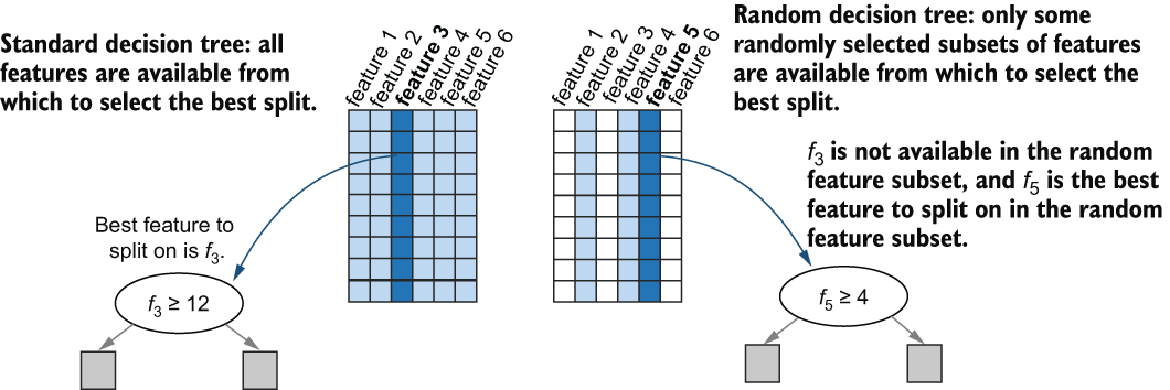
Inspect the split procedure: a node first receives only a subset of columns, then selects the best split within that subset rather than across every feature. section 2.3.1

Training follows a repeated, parallel procedure:

• Draw a bootstrap training subset for one tree. section 2.3.1
• Grow a decision tree, sampling a candidate feature subset before finding the best split at each node. section 2.3.1
• Repeat independently to create many randomized trees. section 2.0
• Aggregate predictions: use majority voting for classification and the mean prediction for regression. section 7.2.1

This two-level randomization—examples through bootstrap sampling and features during tree growth—raises ensemble diversity. Diversity helps reduce variability and smooth predictions. Random forests are therefore a practical off-the-shelf baseline, especially for high-dimensional data, where feature importance rankings can also help identify influential predictive variables. section 2.3 section 2.6

Tree complexity still matters. In scikit-learn, forest estimators accept decision-tree controls such as max_depth and max_leaf_nodes, alongside n_estimators. The implementation supports out-of-bag estimation and parallel execution; setting n_jobs enables use of multiple CPU cores. More trees require more training resources because each base estimator is fully trained, even though the work can be parallelized. section 2.3.2 section 7.2.1

Breast cancer diagnosis: test ensemble size and tree complexity

For Wisconsin Diagnostic Breast Cancer classification, compare bagging with decision trees, random forests, and Extra Trees after preprocessing and a train/test split. Increase n_estimators across repeated runs and average the results to reduce sensitivity to randomness. Training error declines as the ensemble grows; test error declines and then stabilizes. The tree ensembles substantially outperform a single decision tree, illustrating how aggregation can turn unstable trees into robust models that generalize. section 2.5 section 2.5.2

Continuous prediction with RandomForestRegressor

For continuous targets, train regression trees and average their predictions. RandomForestRegressor can use squared-error, absolute-error, or Poisson criteria in the illustrated comparisons. In bike rental prediction, tune n_estimators and max_depth with GridSearchCV, evaluate with cross-validation, and compare test MSE, MAE, and R² against Extra Trees and other models. This keeps loss choice and hyperparameter selection tied to measured predictive performance rather than intuition alone. section 7.2.1 section 7.4.3

Random forests are not the only randomized tree ensemble. Bagging uses bootstrap samples with ordinary decision trees; random forests add feature sampling at each split; Extra Trees also randomize split thresholds and can omit bootstrap sampling. For document retrieval, a LightGBM random-forest configuration can serve as a baseline against gradient-boosting variants, making the speed–accuracy tradeoff explicit. section 2.6 section 5.5.2

How Ensemble Methods for Machine Learning covers it

How deep it goes

Explains bootstrap sampling and per-node feature sampling, then demonstrates scikit-learn training, evaluation, and hyperparameter tuning.

Examples

Uses Wisconsin breast cancer diagnosis, bike rental prediction, split-feature diagrams, and scikit-learn estimator listings.

What it assumes

Assumes familiarity with ensemble learning, bagging, decision trees, train/test splits, and predictive evaluation.

What you can do after

Apply it via scikit-learn by fitting forests, tuning ensemble size and tree depth, and evaluating held-out predictive performance.

How it connects

Connects bagging, decision trees, Extra Trees, feature importance, out-of-bag estimation, and gradient boosting.

liveBookmanning.com

Read Ensemble Methods for Machine Learning on liveBook Get the book at manning.com

Also explained in

• 

  liveBookmanning.com
  Statistics Every Programmer NeedsA random forest is an ensemble model that combines predictions from multiple randomized decision trees.
• 

  liveBookmanning.com
  Grokking Machine LearningAn ensemble model that combines predictions from many decision trees, typically trained with randomized data or feature selection.
• 

  liveBookmanning.com
  Machine Learning for Tabular Data: XGBoost, Deep Learning, and AIAn ensemble of randomized decision trees whose predictions are aggregated.
• 

  liveBookmanning.com
  Outlier Detection in PythonRandom forest is an ensemble learning method that combines predictions from multiple decision trees built using randomized data and feature selection.
• 

  liveBookmanning.com
  Cyber Threat HuntingA random forest is an ensemble machine-learning algorithm that combines predictions from multiple decision trees trained with randomized sampling or feature selection.
• 

  liveBookmanning.com
  Investing for ProgrammersA random forest is an ensemble algorithm that combines predictions from multiple decision trees.
• 

  liveBookmanning.com
  Graph Algorithms for Data ScienceA random forest model is an ensemble of decision trees whose aggregated predictions perform classification or regression.
• 

  liveBookmanning.com
  Data-Driven CybersecurityA random forest is an ensemble machine-learning model that combines predictions from multiple decision trees.
• 

  liveBookmanning.com
  Machine Learning Platform EngineeringA random forest is an ensemble model that combines predictions from multiple decision trees trained with randomized sampling or feature selection.
• 

  liveBookmanning.com
  Financial AI in PracticeA random forest is an ensemble model that combines predictions from multiple decision trees trained with randomized data and feature selection.

Compare how 11 books explain random forest →

Related concepts

• decision treehas part · A decision tree is a branching structure that represents sequential tests or choices, with paths leading to outcomes, predictions, or actions.
• ensemblekind of · An ensemble is a technique that combines or considers outputs from multiple models or component methods collectively to produce or assess a joint result.
• bagginguses · Bagging, or bootstrap aggregation, is an ensemble technique that trains multiple models on bootstrap samples of data and combines their predictions.
• importance scoreuses · An importance score is a numerical value indicating an item's relative significance, relevance, or contribution within a specified context.
• bootstrap samplingused by · Bootstrap sampling is a resampling technique that repeatedly draws observations with replacement from observed data to estimate a statistic’s sampling behavior or variability.

This explainer was generated by Manning's knowledge graph from the text of Ensemble Methods for Machine Learning. The section links point to the parts of the book it draws on.