A standard normal distribution is a bell-shaped normal distribution put on a shared scale: its mean is 0 and its standard deviation is 1. Its horizontal-axis values are Z-scores, so a value says how many standard deviations it sits above or below the mean. That makes measurements with different original units easier to interpret on the same reference curve. section 4.10 section 5.3
Standardizing does not make an unusual observation disappear; it gives its unusualness a number. For an original value x, subtract the distribution mean and divide by its standard deviation. A positive Z-score is above the mean, a negative score is below it, and a score near 0 is close to typical. The conversion can also be reversed to recover an original x-value. section 4.10
Coffee amounts on a Z-scale
Suppose baristas suggest a mean coffee amount of 27.6 grams with a standard deviation of 3.2 grams. A suggestion of 40 grams becomes a Z-score of 3.875: it is 3.875 standard deviations above the mean. Since values within three standard deviations cover 99.7% under the empirical rule, that suggestion is extreme relative to this distribution. section 4.10
The standard normal curve also turns probability questions into area questions. Its total area is 1. For a symmetric middle area of 0.95, the remaining 0.05 is split into two tails of 0.025. The boundary Z-values are the critical Z-values; looking up cumulative areas of 0.025 and 0.975 gives the paired cutoffs, approximately ±1.959964. section 5.3
Figure 5.4 Breaking down the center .95 area in the bell curve and demonstrating the symmetry
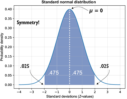
This diagram breaks a central 0.95 area into two equal halves and shows the 0.025 tail left on each side. section 5.3
In hypothesis testing, the same scale provides a home for a test Z-value. A two-tailed test places the significance level across both tails, then asks whether the sample statistic falls beyond the critical region. For tests about means, the standard normal distribution is used here with samples larger than 30, while the t-distribution is preferred for smaller samples and is often used for larger ones too because it represents greater uncertainty. section 6.15 section 6.3
Checking a bag-weight claim
A sample of 41 bags has mean weight 140.2 grams and standard deviation 4.79 grams, compared with an advertised mean of 142 grams. Convert the sample mean into a test Z-value using the sample size and standard deviation, find the two-tailed critical value with a 0.05 significance level, and compare them. The comparison supports either failing to reject or rejecting the claim that the mean is 142 grams; a difference alone is not enough. section 6.6
