Critical z-value

As explained in Grokking Statistics

A cutoff value from a reference distribution that determines the boundary of a statistical confidence interval or decision region.

A critical z-value is a cutoff on the standard normal bell curve. It marks the edge of a chosen central area or, in hypothesis testing, the edge of a tail region considered statistically significant. Think of it as a boundary line: where a z-score lands relative to that line changes the conclusion. section 5.3 section 6.6

Figure 5.4 Breaking down the center .95 area in the bell curve and demonstrating the symmetry

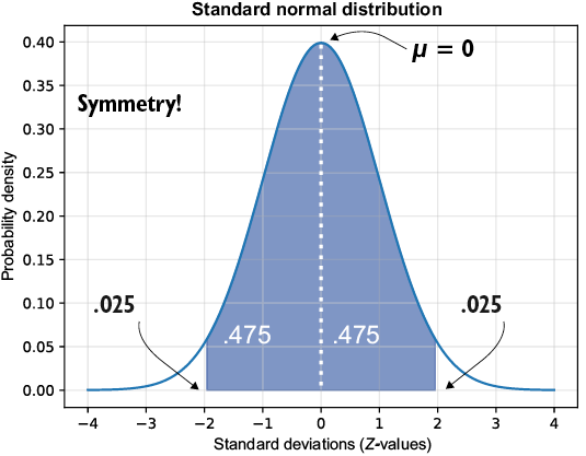
For a two-sided 95% central area, split the remaining 5% evenly: 2.5% sits in each tail. The symmetric boundaries are the critical z-values. section 5.3

For a two-sided confidence interval or test with central area A, find the positive boundary with `norm.ppf(1 - (1 - A) / 2)` and use both `-z` and `+z`. At 95%, the boundaries are approximately ±1.959964. Values beyond those boundaries lie in the two tail areas. section 5.3 section 6.6

Tail choice changes where the cutoff goes:

• In a two-tailed test, split alpha between both tails and reject when the test z-score falls outside the symmetric critical range. section 6.6
• In a left-tailed test, place all alpha in the left tail; at 95% confidence, the critical boundary is about -1.644854. section 6.9
• In a right-tailed test, place all alpha in the right tail; at 95% confidence, the critical boundary is about 1.644854. section 6.9

Potato-chip weight claim

Suppose a bag is claimed to weigh 142 grams on average. With a sample mean of 140.2, sample standard deviation 4.79, and 41 bags, the test z-score is about -2.4062. In a two-tailed test at alpha = 0.05, it falls outside [-1.959964, 1.959964], so reject the claim. In a left-tailed test, it also falls beyond the -1.64485 cutoff. A cutoff supports a decision under the chosen rule; it is not automatic proof of a real-world claim. section 6.6 section 6.10

Critical z-values also power confidence intervals: the central area selected on the standard normal curve helps define a range used to estimate a population mean or proportion from a sample. Smaller samples estimating a mean may instead call for the t-distribution. section 5.9 section 5.2

How Grokking Statistics covers it

How deep it goes

Works through symmetric-area and tail calculations with PPF code, without deriving normal-distribution formulas.

Examples

Uses golden retriever sample weights and a 142-gram potato-chip bag claim, with 95% two- and one-tailed cutoffs.

What it assumes

Introduces standard normal z-scores and probability areas before tying them to confidence intervals and tests.

What you can do after

Apply it via SciPy's normal PPF to calculate critical boundaries and compare test z-scores with rejection regions.

How it connects

Connects confidence intervals, standard normal distribution, z-scores, cumulative distribution functions, significance levels, null hypotheses, and t-distribution.

liveBookmanning.com

Read Grokking Statistics on liveBook Get the book at manning.com

Related concepts

• confidence intervalconfigures · A confidence interval is a range estimated from data by a statistical procedure designed to provide a specified long-run coverage probability for an unknown quantity.
• margin of erroruses · A margin of error is a bound or tolerance representing the expected uncertainty or deviation around an estimate, measurement, prediction, or result.
• standard normal distributionused by · A standard normal distribution is a normal probability distribution with mean zero and standard deviation one.
• one-sided testconfigured by · A one-sided test is a hypothesis test whose alternative hypothesis and rejection region concern a departure from the null in one prespecified direction.
• inverse cumulative density functionuses · An inverse cumulative distribution function maps a cumulative probability to the corresponding value of a random variable.
• z-scoreconfigures · A z-score is a signed standardized value expressing how many standard deviations an observation lies above or below a reference mean.

This explainer was generated by Manning's knowledge graph from the text of Grokking Statistics. The section links point to the parts of the book it draws on.