An adjacency matrix records relationships between pairs of nodes. Rows and columns identify nodes; an entry indicates whether the corresponding pair is connected. In political districting, nodes are neighborhoods and the matrix records which neighborhoods meet the chosen geographic test. The same representation can supply graph structure to a graph neural network. section 8.8 section 11.3.1
Build one from neighborhood geometry
For each neighborhood, inspect every other neighborhood. Put 1 in the matrix when their geometries intersect, and leave 0 otherwise. The implementation skips pairs with the same index, so its diagonal remains zero. Its intersection test is the operative definition of “neighbor”; choose that test to match the districting problem. section 8.8
import numpy as np

def get_population(lst, table):
    return table["population"].iloc[lst].to_numpy()    #1

eval = get_population(range(range_limit), values)      #2

def get_neighboors(database):                          #3
    result = []
    for i in range(database['name'].size):
        tmp = np.zeros(database['name'].size)
        geo1 = database.iloc[i]
        for j in range(database['name'].size):
            if i != j:
                geo2 = database.iloc[j]
                if geo1["geometry"].intersects(geo2["geometry"]):
                    tmp[j] = 1
        result.append(tmp)
    return np.stack(result)

neighbor = get_neighboors(toronto_sample)
The NumPy and GeoPandas listing shows the pairwise geometry checks and the resulting zero–one matrix. section 8.8
The districting problem passes this matrix alongside neighborhood populations and the number of districts to a genetic-algorithm optimization. Its constraint calculations use matrix operations to test neighborhood relationships in candidate district assignments. Building the matrix with a nested loop checks every ordered pair, so the preprocessing work grows with the square of the neighborhood count. section 8.8
The entries play different roles in graph learning:
- A graph convolutional network uses an unweighted adjacency matrix with node features to produce embeddings through neighboring-node message passing. section 11.3.1
- A graph attention network weights neighboring nodes by attention coefficients; attention remains restricted to the node’s neighborhood. section 11.3.2
- A supervised traveling-salesman pipeline begins with node features and an adjacency matrix, then uses graph embeddings and predicted solution probabilities to guide graph search. section 11.7
Figure 11.9 Graph convolutional network (GCN) vs. graph attention network (GAT)
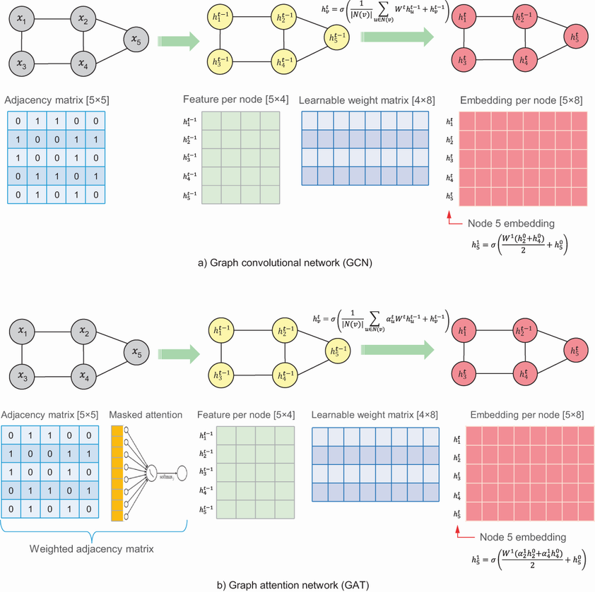
The comparison figure distinguishes unweighted graph convolution from attention-weighted neighbor contributions. section 11.3.2