A sequence-to-sequence RNN can compress an input sentence into one context vector. Its output then lacks direct access to individual input words. Attention removes this bottleneck: for each output, it forms a context vector by weighting the input word vectors according to their relevance. section 11.3
More generally, attention is a soft dictionary lookup. Let each query qᵢ search candidate keys kⱼ, with a value vⱼ attached to each key. A scoring function measures how well each key matches the query; normalizing those scores produces weights aᵢⱼ that sum to one. The result for query i is the weighted sum Σⱼ aᵢⱼvⱼ. Unlike an exact lookup, several values can contribute to one result. section 11.3
One scoring choice uses a trainable matrix W to compare queries and keys; a normalized multiplicative choice uses W = 1. With queries and keys arranged as matrices Q and K, that choice gives A = softmax(QKᵀ), with softmax applied across the candidate keys for each query. The output is AV, where V holds the corresponding values. Each row of A therefore says where one query looks in V. section 11.3
Figure 11.9 Attention matrix heatmap for neural machine translation
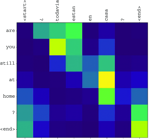
The neural-machine-translation heatmap makes the weight matrix concrete: target-sequence queries distribute attention over source-sequence words. section 11.3
Self-attention is a key component of transformers, which use attention in both encoder and decoder. A text-classification implementation provides a practical setting for working with a transformer architecture in Keras/TensorFlow. section 11.7 section 11.3
Listing 11.3 Transformer for text classification
import numpy as np
import pandas as pd

import tensorflow as tf
from tensorflow import keras

from keras.models import Model, Sequential
from keras.layers import Layer, Dense, Dropout, Activation
from keras.layers import LayerNormalization, MultiHeadAttention
from keras.layers import Input, Embedding, GlobalAveragePooling1D

from keras import regularizers
from keras.preprocessing import sequence
from keras.utils import np_utils

from keras.callbacks import ModelCheckpoint
from keras.callbacks import TensorBoard
from keras.callbacks import LearningRateScheduler
from keras.callbacks import EarlyStopping

import matplotlib.pyplot as plt

tf.keras.utils.set_random_seed(42)

SAVE_PATH = "/content/drive/MyDrive/Colab Notebooks/data/"

def scheduler(epoch, lr):   #1
    if epoch < 4:
        return lr
    else:
        return lr * tf.math.exp(-0.1)

#load dataset
max_words = 20000     #2
seq_len = 200     #3
(x_train, y_train), (x_val, y_val) =
 keras.datasets.imdb.load_data(num_words=max_words)

x_train = keras.utils.pad_sequences(x_train, maxlen=seq_len)
x_val = keras.utils.pad_sequences(x_val, maxlen=seq_len)

class TransformerBlock(Layer):
    def __init__(self, embed_dim, num_heads, ff_dim, rate=0.1):
        super(TransformerBlock, self).__init__()
        self.att = MultiHeadAttention(num_heads=num_heads, key_dim=embed_dim)
        self.ffn = Sequential(
            [Dense(ff_dim, activation="relu"), Dense(embed_dim)]
        )
        self.layernorm1 = LayerNormalization(epsilon=1e-6)
        self.layernorm2 = LayerNormalization(epsilon=1e-6)
        self.dropout1 = Dropout(rate)
        self.dropout2 = Dropout(rate)

    def call(self, inputs, training):
        attn_output = self.att(inputs, inputs)
        attn_output = self.dropout1(attn_output, training=training)
        out1 = self.layernorm1(inputs + attn_output)
        ffn_output = self.ffn(out1)
        ffn_output = self.dropout2(ffn_output, training=training)
        return self.layernorm2(out1 + ffn_output)

class TokenAndPositionEmbedding(Layer):
    def __init__(self, maxlen, vocab_size, embed_dim):
        super(TokenAndPositionEmbedding, self).__init__()
        self.token_emb = Embedding(input_dim=vocab_size,
         output_dim=embed_dim)
        self.pos_emb = Embedding(input_dim=maxlen, output_dim=embed_dim)

    def call(self, x):
        maxlen = tf.shape(x)[-1]
        positions = tf.range(start=0, limit=maxlen, delta=1)
        positions = self.pos_emb(positions)
        x = self.token_emb(x)
        return x + positions

batch_size = 32
num_epochs = 8     #4

embed_dim = 32     #5
num_heads = 2   #5
ff_dim = 32      #5

#transformer architecture
inputs = Input(shape=(seq_len,))
embedding_layer = TokenAndPositionEmbedding(seq_len, max_words, embed_dim)
x = embedding_layer(inputs)
transformer_block = TransformerBlock(embed_dim, num_heads, ff_dim)
x = transformer_block(x)
x = GlobalAveragePooling1D()(x)
x = Dropout(0.1)(x)
x = Dense(20, activation="relu")(x)
x = Dropout(0.1)(x)
outputs = Dense(2, activation="softmax")(x)

model = Model(inputs=inputs, outputs=outputs)

model.compile(
  loss=keras.losses.SparseCategoricalCrossentropy(),
  optimizer=tf.keras.optimizers.Adam(),
  metrics=["accuracy"]
)

#define callbacks
file_name = SAVE_PATH + 'transformer-weights-checkpoint.h5'
#checkpoint = ModelCheckpoint(file_name, monitor='val_loss', verbose=1,
 save_best_only=True, mode='min')
reduce_lr = LearningRateScheduler(scheduler, verbose=1)
early_stopping = EarlyStopping(monitor='val_loss', min_delta=0.01,
 patience=16, verbose=1)
#tensor_board = TensorBoard(log_dir='./logs', write_graph=True)
callbacks_list = [reduce_lr, early_stopping]

hist = model.fit(x_train, y_train, batch_size=batch_size,
 epochs=num_epochs, callbacks=callbacks_list, validation_data=(x_val,
 y_val))     #6

test_scores = model.evaluate(x_val, y_val, verbose=2) #7

print("Test loss:", test_scores[0])
print("Test accuracy:", test_scores[1])

plt.figure()
plt.plot(hist.history['loss'], 'b', lw=2.0, label='train')
plt.plot(hist.history['val_loss'], '--r', lw=2.0, label='val')
plt.title('Transformer model')
plt.xlabel('Epochs')
plt.ylabel('Cross-Entropy Loss')
plt.legend(loc='upper right')
plt.show()

plt.figure()
plt.plot(hist.history['accuracy'], 'b', lw=2.0, label='train')
plt.plot(hist.history['val_accuracy'], '--r', lw=2.0, label='val')
plt.title('Transformer model')
plt.xlabel('Epochs')
plt.ylabel('Accuracy')
plt.legend(loc='upper left')
plt.show()

plt.figure()
plt.plot(hist.history['lr'], lw=2.0, label='learning rate')
plt.title('Transformer model')
plt.xlabel('Epochs')
plt.ylabel('Learning Rate')
plt.legend()
plt.show()
The transformer text-classification listing shows the practical Keras/TensorFlow implementation, including its use of a MultiHeadAttention layer. section 11.3