A Bézier curve is a flexible parametric curve drawn from endpoints and control points. Its shape can be rendered at variable precision, making it useful when graph edges need smoother alternatives to polylines. section 15.4.3 section 15.4
Construct a quadratic curve from endpoints S and E and control point C1. For a parameter t from 0 to 1, choose proportional points A and B on SC1 and EC1, then choose Pt on AB using the same ratio. The collection of Pt values forms the curve, with Pt equal to an endpoint when t is 0 or 1. section 15.4.3
Figure 15.21 How a quadratic Bézier curve is drawn. A quadratic curve requires three points: two endpoints (S, E) and a control point (C1, or just C for the sake of clarity here henceforth). First we have to draw the two segments between the endpoints and C. Then, we can draw segments whose endpoints are on SC and EC, under the constraint that if the endpoint on the former, call it A, is such that SA/SC=t, then B, the remaining endpoint, must satisfy EB/EC=(1-t). Finally, on segment AB, we choose a point P such that AP/AB=t.
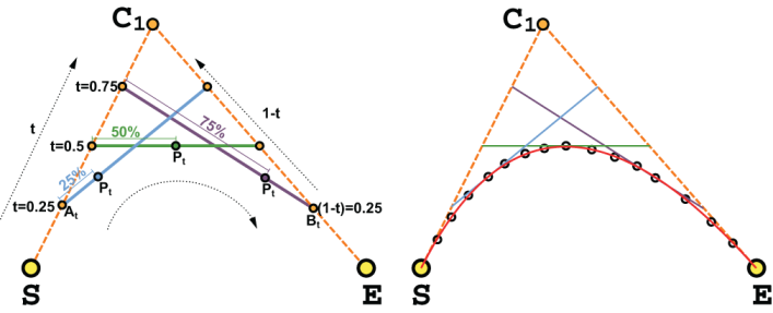
Follow the three-stage construction from the endpoints and control point to the moving point Pt; the intermediate segment remains tangent to the curve. section 15.4.3
Choose the curve variant according to the flexibility and parameter count required:
- Use a quadratic curve with two endpoints and one control point. section 15.4.3
- Use a cubic curve with two endpoints and two control points when greater flexibility is needed. section 15.4.3 section 16.1.2
- Restrict quadratic curves to symmetric control points when balancing flexibility against simpler intersection handling; one real distance parameter can describe the shape. section 15.4.4 section 16.1.2
Checking curved-edge intersections
Compare the curves’ convex hulls first. If they do not overlap, the curves cannot intersect; otherwise, subdivide them repeatedly until the remaining pieces are small enough to approximate with line segments within an acceptable error. section 15.4.4