A Bézier curve is a parametric polynomial curve built from control points and basis functions. It is a practical model for the smooth lines once shaped with flexible metal splines, now common in graphic design, games, GIS, virtual reality, CAD, and manufactured objects. section 7.0 section 7.2.3
Use a parameter t from 0 to 1 to travel along the curve. In 2D, evaluate one Bézier function for x and another for y; in 3D, add a third coordinate function. Rather than solve directly for polynomial coefficients, combine polynomial basis functions with coordinate values from the control points. section 7.2.3
The first-degree case is linear interpolation: B¹(t) = (1 − t)y₁ + ty₂. At t = 0 it returns y₁, and at t = 1 it returns y₂. The two terms, 1 − t and t, are basis polynomials whose changing weights move the result from one endpoint to the other. section 7.2.3
Higher degrees add shape control while retaining endpoint behavior:
- A quadratic curve uses three control points. It starts and ends at the outer points; the middle point shapes the curve rather than necessarily lying on it. section 7.2.3
- A cubic curve uses four control points, with two interior points controlling its shape. section 7.2.3
- Control points set tangents indirectly, unlike explicit polynomial modeling, where tangents are specified directly. section 7.2.4
Quadratic coordinate evaluation
For control-point coordinates xs = [0, 0.3, 1], evaluate x(t) = (1−t)²xs[0] + 2(1−t)txs[1] + t²xs[2]. Apply the identical calculation to ys = [0.2, 0.8, 0.5] to obtain y(t), then pair x(t) and y(t) to plot the curve. section 7.2.3
Classic Bézier functions are weighted sums of polynomial bases and therefore remain polynomials. Rational Bézier functions add control-point weights through a numerator-and-denominator calculation; changing weights reshapes a curve without changing its control points. Rationality also permits exact conic sections, including ellipses and hyperbolas. section 7.2.3 section 7.6
Figure 7.18 Cubic Bézier curves with the same control points with different weights, from left to right and top to bottom: (1, 1, 1, 1), (1, 2, 2, 1), (1, 0, 0, 1), (1, 1, 4, 1)
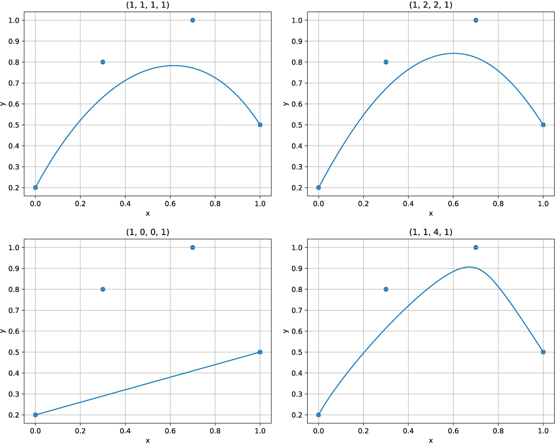
Compare cubic curves made from identical control points but different weights to see how rational Bézier weighting changes the shape. section 7.2.3
For longer shapes, join Bézier pieces into a spline. A Bézier function is defined on [0,1], and a Bézier spline is uniform: each piece has the same parametric distance. NURBS extend Bézier curves with rationality and nonuniform knot vectors, letting selected control points interpolate the curve while others shape it. section 7.3.2 section 11.1
Bézier pieces also provide a final smoothing step for contours initially represented by line segments. When fitting such contours, an approximation threshold trades accuracy against iteration count and speed: a lower threshold improves fit but requires more iterations. section 12.4.3