Will it rain today? A forecast is more useful when it expresses uncertainty than when it simply says “rain” or “no rain.” Bayesian statistics uses probability to represent what is known about an unknown quantity, then revises that belief when new evidence arrives. The result is a probability distribution, not just a single prediction. section 1.0 section 1.5
A Bayesian update has three parts:
- A prior distribution expresses beliefs about the possible values before seeing the new data. section 2.0 section 2.15
- A likelihood describes how probable the observed data would be under each possible value or hypothesis. section 2.15
- A posterior distribution combines the prior and likelihood: multiply their corresponding probabilities, then normalize the results so they sum to 1. section 2.15
A dark cloud changes a forecast
Suppose the prior chance of rain is 0.1. A dark cloud is likely on a rainy day (0.99), but it can also appear on a dry day (0.2). The two unnormalized weights are 0.1 × 0.99 = 0.099 for rain and 0.9 × 0.2 = 0.18 for no rain. Divide each by their sum, 0.279. The updated chance of rain is about 0.355: higher than before, yet no rain remains more likely. Evidence matters, but so does the starting belief. section 2.4
The same reasoning helps interpret a positive test for a rare disease. Ignoring how rare the disease is can make the result seem more conclusive than it is. As further evidence arrives, the current posterior can become the prior for the next update. section 2.5
A distribution also shows uncertainty about an estimate. If three of five surveyed coworkers prefer tea, 0.6 is a simple estimate of the wider group’s preference, but five responses leave considerable uncertainty. More survey responses can make the posterior more concentrated. When a posterior cannot be calculated in closed form, Monte Carlo sampling can approximate it for predictions, credible intervals, and decisions. section 2.8 section 2.13 section 5.0
Figure 2.4 Comparison between the prior and posterior distributions of 𝑝 under different datasets. As the size of the dataset grows, the most-likely prediction of 𝑝 becomes more confident.
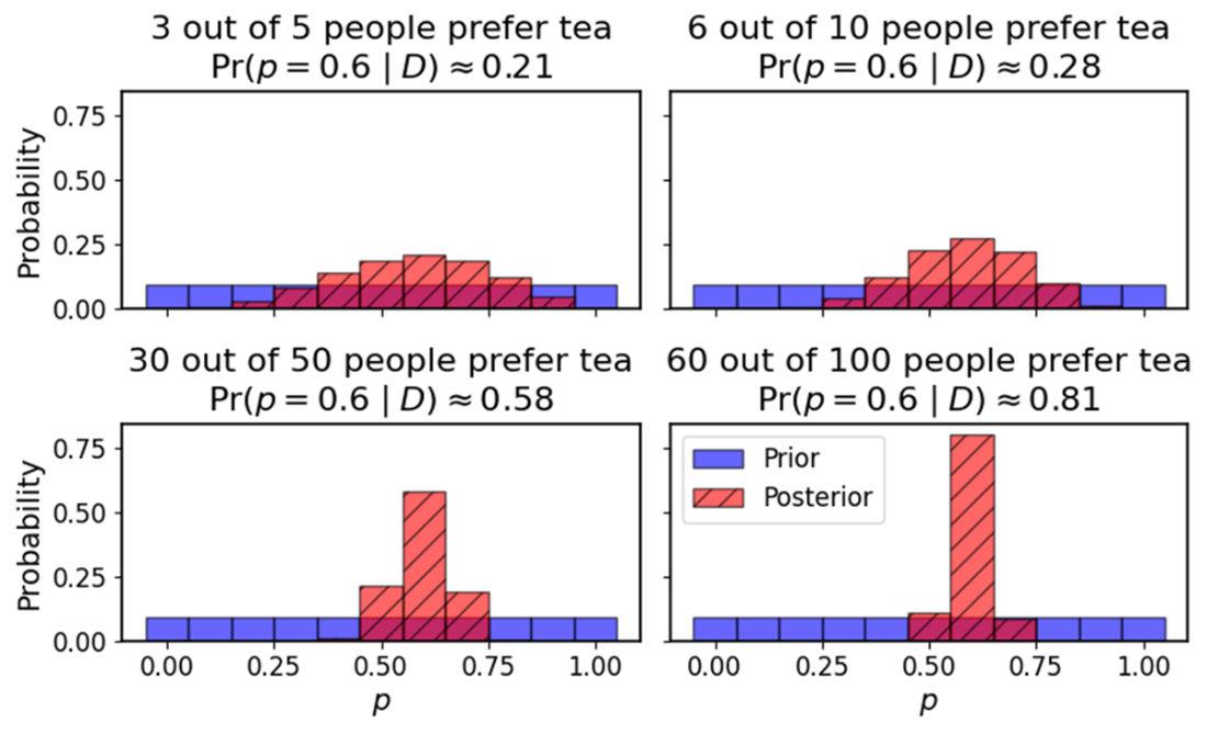
Compare the posterior distributions for surveys of 5, 10, 50, and 100 people; each has the same observed proportion, but larger samples yield greater confidence. section 2.13